From the free course Statistics and Probability on Lykke
Chi-Square Tests
Key concepts: Goodness-of-Fit Test · Test for Independence · Test for Homogeneity · Expected Counts · Degrees of Freedom
Using Chi-Square distributions to analyze categorical data in two-way tables.
Chi-Square Tests
The Chi-Square ($\chi^2$) test family represents a cornerstone of non-parametric statistics, providing a robust framework for analyzing categorical data. While the t-test and ANOVA dominate the landscape of quantitative variables (means and variances), the Chi-Square test allows us to rigorously evaluate frequencies, proportions, and associations. Developed primarily by Karl Pearson at the turn of the 20th century, these tests bridge the gap between observed reality and theoretical expectation.
The Mathematical Foundation: The $\chi^2$ Distribution
Before diving into specific tests, we must understand the distribution itself. The Chi-Square distribution with $k$ degrees of freedom is the distribution of a sum of the squares of $k$ independent standard normal random variables. Mathematically, if $Z_1, Z_2, \dots, Z_k$ are independent $N(0, 1)$ variables, then:
$$Q = \sum_{i=1}^{k} Z_i^2 \sim \chi^2(k)$$
The distribution is characterized by its Degrees of Freedom (df), which dictates its shape. Unlike the symmetric Normal distribution, the $\chi^2$ distribution is skewed to the right, though it approaches normality as $df$ increases.
The Fundamental Statistic
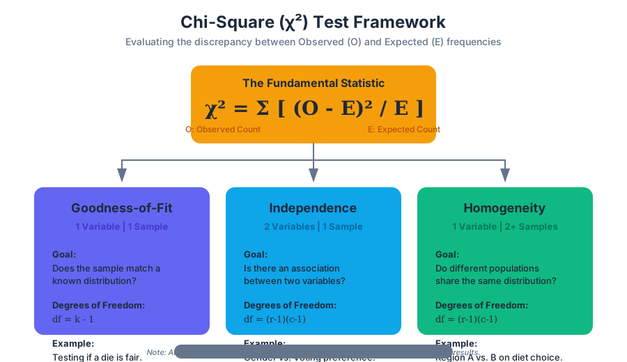
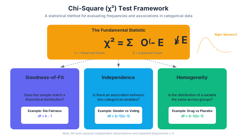
Regardless of the specific test type, the core mechanic involves calculating the Chi-Square Statistic, denoted as $\chi^2$. This value quantifies the "distance" between what we actually saw (Observed counts) and what we would expect to see if the null hypothesis were true (Expected counts).
$$\chi^2 = \sum \frac{(O - E)^2}{E}$$
Where:
- $O$: The observed frequency in a category.
- $E$: The expected frequency in a category under $H_0$.
The Intuition of the Formula: We square the difference $(O-E)$ to ensure that positive and negative deviations don't cancel each other out. We divide by $E$ to normalize the deviation; a difference of 10 is massive if you expected 5, but negligible if you expected 5,000.
1. Chi-Square Goodness-of-Fit (GoF) Test
The Goodness-of-Fit Test is used to determine if a sample of categorical data matches a specific population distribution. It is a "one-variable" test.
When to Use It
- To check if a die is fair (uniform distribution).
- To see if the ethnic breakdown of a jury matches the census data of a city.
- To verify if Mendelian genetics (e.g., a 3:1 ratio) holds for a cross-breeding experiment.
Mechanics and Degrees of Freedom
In a GoF test, the degrees of freedom are calculated as: $$df = k - 1$$ where $k$ is the number of categories. We lose one degree of freedom because the total count is fixed; if you know the counts of $k-1$ categories, the last one is determined.
2. Chi-Square Test for Independence
The Test for Independence evaluates whether there is a significant association between two categorical variables in a single population. It asks: "Does the value of Variable A depend on the value of Variable B?"
The Contingency Table
Data for this test is organized into a $r \times c$ contingency table (or two-way table), where $r$ is the number of rows and $c$ is the number of columns.
| Variable A \ Variable B | Category B1 | Category B2 | Row Totals |
|---|---|---|---|
| Category A1 | $O_{11}$ | $O_{12}$ | $R_1$ |
| Category A2 | $O_{21}$ | $O_{22}$ | $R_2$ |
| Column Totals | $C_1$ | $C_2$ | N |
Calculating Expected Counts
Under the assumption of independence, the probability of an observation falling into cell $(i, j)$ is the product of the marginal probabilities. Therefore, the expected count for any cell is:
$$E_{i,j} = \frac{(\text{Row } i \text{ Total}) \times (\text{Column } j \text{ Total})}{\text{Grand Total (N)}}$$
Mathematical Derivation of Expected Values
The derivation relies on the definition of independent events: $P(A \cap B) = P(A) \times P(B)$.
% Logic for Expected Value in Independence Test
P(Row_i) = Row_i_Total / N
P(Col_j) = Col_j_Total / N

Assuming Independence:
P(Row_i AND Col_j) = (Row_i_Total / N) * (Col_j_Total / N)

Expected Count (E_ij):
E_ij = N * P(Row_i AND Col_j)
E_ij = N * (Row_i_Total / N) * (Col_j_Total / N)
E_ij = (Row_i_Total * Col_j_Total) / N
3. Chi-Square Test for Homogeneity
While the Test for Independence looks at two variables in one population, the Test for Homogeneity looks at one variable across multiple populations (or treatment groups).
Key Distinction
- Independence: One sample, two variables. (e.g., Sample 500 voters; ask their party and their gender).
- Homogeneity: Multiple samples, one variable. (e.g., Sample 200 men and 200 women separately; ask if they support a specific policy).
Mathematically, the calculation for the $\chi^2$ statistic and the degrees of freedom are identical to the test for independence. The difference lies entirely in the sampling design and the null hypothesis statement.
| Feature | Test for Independence | Test for Homogeneity |
|---|---|---|
| Goal | See if Variable X and Y are related. | See if Group A and B have the same distribution. |
| Sampling | Single random sample. | Multiple independent random samples. |
| Null Hypothesis | Variable A and B are independent. | The distribution of Variable X is the same across populations. |
| Degrees of Freedom | $(r-1)(c-1)$ | $(r-1)(c-1)$ |
4. Degrees of Freedom and Critical Values
The Degrees of Freedom (df) represent the number of values in the final calculation of a statistic that are free to vary.
Summary of df Calculations
| Test Type | Formula | Explanation |
|---|---|---|
| Goodness-of-Fit | $k - 1$ | $k$ is the number of levels/categories. |
| Independence | $(r-1)(c-1)$ | $r$ = rows, $c$ = columns in the table. |
| Homogeneity | $(r-1)(c-1)$ | $r$ = number of populations, $c$ = category levels. |
5. Assumptions and Conditions
The Chi-Square test is powerful, but it is not "distribution-free" in the sense that it requires specific conditions to be valid. If these are violated, the $\chi^2$ approximation to the sampling distribution of the test statistic fails.
- Randomness: The data must come from a random sample or a randomized experiment.
- Independence: Each observation must be independent of others. This means the sample size $n$ should be less than 10% of the population if sampling without replacement.
- Large Sample Size (Cochran's Rule):
- All Expected Counts must be at least 1.
- At least 80% of Expected Counts must be at least 5.
- Note: If these are not met, use Fisher's Exact Test (for $2 \times 2$ tables) or collapse categories.
6. Worked Example: Independence Test
Scenario: A tech company wants to know if the choice of Operating System (OS) is independent of the user's job role. They survey 200 employees.
Step 1: State Hypotheses
- $H_0$: OS choice and Job Role are independent.
- $H_a$: OS choice and Job Role are dependent.
Step 2: Observed Data (Contingency Table)
| MacOS | Windows | Linux | Total | |
|---|---|---|---|---|
| Devs | 40 | 20 | 40 | 100 |
| Designers | 70 | 20 | 10 | 100 |
| Total | 110 | 40 | 50 | 200 |
Step 3: Calculate Expected Counts
For Devs/MacOS: $E = (100 \times 110) / 200 = 55$ For Designers/Linux: $E = (100 \times 50) / 200 = 25$ (And so on for all 6 cells)
Step 4: Compute $\chi^2$
$$\chi^2 = \frac{(40-55)^2}{55} + \frac{(20-20)^2}{20} + \dots$$ After calculation, suppose $\chi^2 = 32.7$.
Step 5: Determine P-value
With $df = (2-1)(3-1) = 2$, a $\chi^2$ of 32.7 yields a p-value $< 0.0001$. Conclusion: Reject $H_0$. There is a significant association between job role and OS preference.
7. Common Pitfalls and Misconceptions
Pitfall 1: Using Percentages instead of Counts
The Chi-Square formula $\sum \frac{(O-E)^2}{E}$ is strictly defined for frequencies (counts). Using percentages or proportions will result in an incorrect (usually much smaller) $\chi^2$ value, leading to Type II errors (failing to reject a false null).
Pitfall 2: Confusing Independence and Homogeneity
While the math is the same, the interpretation differs. If you sampled 100 people and asked two questions, it's Independence. If you sampled 50 men and 50 women and asked one question, it's Homogeneity.
Pitfall 3: Ignoring the "Small Cell" Problem
When expected counts are too low, the $\chi^2$ statistic becomes unstable. In a $2 \times 2$ table, some researchers use the Yates' Continuity Correction, though modern statisticians often prefer Fisher's Exact Test.
Pitfall 4: Correlation vs. Causation
A significant Chi-Square result for independence shows an association, not causality. Just because "Ice Cream Flavor" and "Sunburn Severity" might be dependent doesn't mean mint chocolate chip causes skin damage; both are likely dependent on a third variable (Temperature/Season).
Summary of Chi-Square Variants
| Test Name | Number of Variables | Number of Populations | Null Hypothesis ($H_0$) |
|---|---|---|---|
| Goodness-of-Fit | 1 | 1 | The sample follows the specified distribution. |
| Independence | 2 | 1 | The two variables are not related. |
| Homogeneity | 1 | 2+ | The distribution is the same across all populations. |
Source Materials
Study Statistics and Probability on Lykke
This course page is free to open: signed out, you can read its first two sections, and signing in, on any plan, opens the rest. The free Lykke Chrome extension syncs your own Canvas courses, so ChatGPT, Claude and Muse can answer from your classes and deadlines. It only reads Canvas.
Add the free extensionSign in to open every sectionAll sections of Statistics and Probability · Browse more course pages