From the free course Statistics and Probability on Lykke
Analyzing Categorical Data
Key concepts: Categorical vs. Quantitative Variables · Two-Way Frequency Tables · Marginal and Conditional Distributions · Data Visualization (Bar Graphs, Pie Charts)
Introduction to identifying variables and visualizing categorical data using frequency tables and charts.
Analyzing Categorical Data
In the rigorous study of statistics, data is the raw material from which we forge insight. However, not all data is created equal. Before we can apply the machinery of hypothesis testing or predictive modeling, we must first understand the fundamental nature of the variables we are observing. The analysis of categorical data—information that sorts individuals into distinct groups or categories—serves as the gateway to understanding qualitative relationships, social structures, and logical associations.
While quantitative data deals with "how much" or "how many," categorical data addresses "what kind." This section explores the taxonomies of data, the mechanics of frequency distributions, and the mathematical frameworks used to identify associations between non-numerical variables.
Categorical vs. Quantitative Variables
The first step in any data analysis pipeline is variable classification. A variable is any characteristic, number, or quantity that can be measured or counted.
Categorical Variables
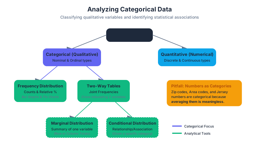
A categorical variable (also known as a qualitative variable) places an individual into one of several groups or categories. These categories may have a natural order (ordinal), such as "low, medium, high," or they may be purely nominal, such as "hair color" or "zip code."
Note on Numbers as Categories: It is a common pitfall to assume that any numerical value is quantitative. Zip codes, area codes, and jersey numbers are categorical because performing arithmetic on them (e.g., calculating the "average" zip code) yields a meaningless result.
Quantitative Variables
A quantitative variable takes numerical values for which it makes sense to find an average. These are further divided into discrete (countable values, like the number of children) and continuous (values that can take any real number within an interval, like height or time).
| Feature | Categorical (Qualitative) | Quantitative (Numerical) |
|---|---|---|
| Data Type | Labels, Names, Categories | Counts, Measurements |
| Operations | Counting, Proportions, Mode | Mean, Median, Standard Deviation |
| Sub-types | Nominal, Ordinal | Discrete, Continuous |
| Example | Species, Blood Type, Rating (1-5) | Weight, Temperature, Population |
| Visualization | Bar Graphs, Pie Charts | Histograms, Box Plots, Scatter Plots |
Frequency and Relative Frequency
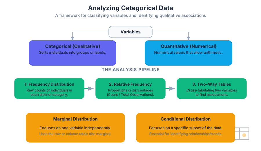
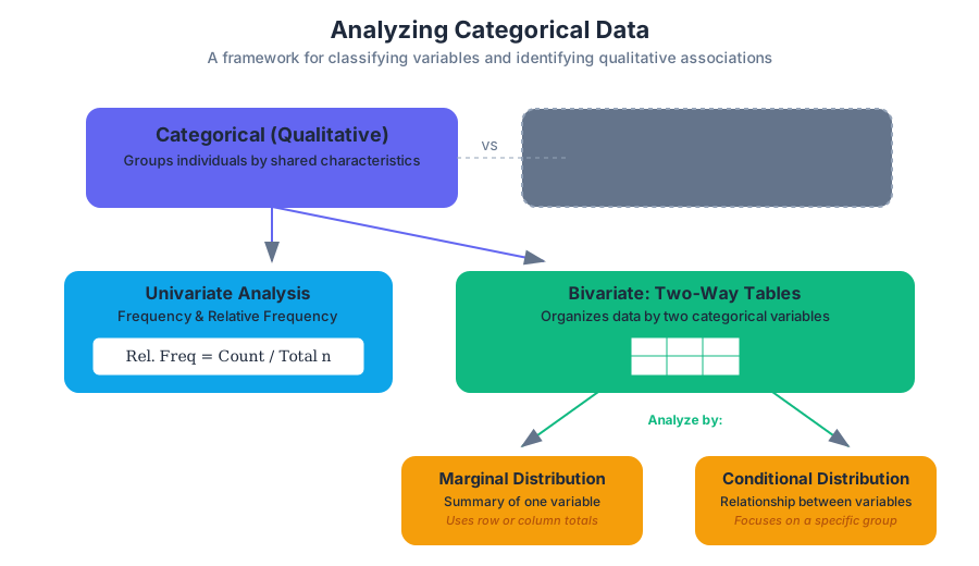
To analyze a single categorical variable, we begin by counting how many individuals fall into each category. This is known as a frequency distribution. However, raw counts can be misleading when comparing groups of different sizes. To normalize the data, we use relative frequency, which expresses the count as a proportion or percentage of the total.
$$\text{Relative Frequency} = \frac{\text{Count in Category}}{\text{Total Number of Observations}}$$
Visualization: Bar Graphs and Pie Charts
- Bar Graphs: These represent each category as a bar whose height corresponds to the frequency or relative frequency. They are superior to pie charts because the human eye is better at comparing linear lengths than angular areas.
- Pie Charts: These show the distribution of a categorical variable as "slices" of a circle. They are only appropriate when you want to emphasize a category's relation to the whole (100%).
Two-Way Frequency Tables
When we wish to examine the relationship between two categorical variables, we employ a two-way table (also called a contingency table or cross-tabulation). This structure allows us to summarize data for the same group of individuals across two different characteristics.
Structure of a Two-Way Table
Consider a study examining the relationship between "Exercise Habit" (Regular, Occasional, Never) and "Sleep Quality" (Good, Poor).
| Good Sleep | Poor Sleep | Total (Marginal) | |
|---|---|---|---|
| Regular Exercise | 45 | 15 | 60 |
| Occasional Exercise | 30 | 35 | 65 |
| Never Exercise | 10 | 65 | 75 |
| Total (Marginal) | 85 | 115 | 200 |
In this table:
- The cells in the interior contain the joint frequencies.
- The row totals and column totals represent the marginal distributions.
Marginal Distributions
The marginal distribution of one of the categorical variables in a two-way table is the distribution of values of that variable among all individuals described by the table. We call it "marginal" because the totals typically appear in the right or bottom margins of the table.
To calculate the marginal distribution for "Exercise Habit" from the table above:
- Identify the row totals for each exercise category.
- Divide each row total by the grand total (200).
| Exercise Habit | Frequency | Relative Frequency |
|---|---|---|
| Regular | 60 | $60/200 = 0.30$ (30%) |
| Occasional | 65 | $65/200 = 0.325$ (32.5%) |
| Never | 75 | $75/200 = 0.375$ (37.5%) |
Key Insight: Marginal distributions tell us nothing about the relationship between the two variables. They only summarize each variable independently.
Conditional Distributions
To understand the association between variables, we must look at conditional distributions. A conditional distribution describes the values of one variable among individuals who have a specific value of another variable.
Mathematically, the conditional distribution of variable $Y$ given $X = x$ is: $$P(Y | X=x) = \frac{\text{Frequency of } (X=x \text{ and } Y)}{\text{Total Frequency of } X=x}$$
Worked Example: Sleep Quality Given Exercise
Let’s find the conditional distribution of Sleep Quality for those who "Regularly Exercise."
- Total Regular Exercisers: 60
- Regular Exercisers with Good Sleep: 45 ($45/60 = 75%$)
- Regular Exercisers with Poor Sleep: 15 ($15/60 = 25%$)
Now, compare this to those who "Never Exercise":
- Total Never Exercisers: 75
- Never Exercisers with Good Sleep: 10 ($10/75 \approx 13.3%$)
- Never Exercisers with Poor Sleep: 65 ($65/75 \approx 86.7%$)
Identifying Independence and Association
The primary goal of analyzing two-way tables is to determine if there is an association between two variables.
Definition of Independence: Two categorical variables are independent if the conditional distributions of one variable are the same for all categories of the other variable.
If the conditional distribution of "Good Sleep" is significantly higher for "Regular Exercisers" (75%) than for those who "Never Exercise" (13.3%), we conclude there is a strong association between exercise and sleep quality. If the percentages were nearly identical (e.g., 40% for both), the variables would be considered independent.
Visualizing Association: Segmented Bar Graphs
A segmented bar graph (or stacked bar graph) is the gold standard for visualizing associations. Each bar represents a category of the explanatory variable, and the bar is divided into segments representing the proportions of the response variable. If the segments vary in height across the bars, an association is present.
Implementation and Computation
In modern data science, we rarely calculate these distributions by hand. We use computational libraries to generate contingency tables and perform statistical tests like the Chi-Square test for independence.
2. Mathematical Derivation (LaTeX)
The logic of categorical analysis is rooted in probability theory. We define the relationship between joint, marginal, and conditional probabilities as follows:
\begin{aligned}
&\text{Let } A \text{ and } B \text{ be two categorical variables.} \\
&\text{Joint Probability: } P(A_i \cap B_j) = \frac{n_{ij}}{N} \\
&\text{Marginal Probability: } P(A_i) = \sum_{j} P(A_i \cap B_j) = \frac{n_{i \cdot}}{N} \\
&\text{Conditional Probability: } P(B_j | A_i) = \frac{P(A_i \cap B_j)}{P(A_i)} = \frac{n_{ij}}{n_{i \cdot}} \\
&\text{Independence Condition: } P(B_j | A_i) = P(B_j) \text{ for all } i, j
\end{aligned}
Advanced Nuance: Simpson's Paradox
An expert-level analysis of categorical data must account for Simpson's Paradox. This occurs when an association between two variables reverses or disappears when a third "lurking" or "confounding" variable is introduced.
The Classic Example: University Admissions
Imagine a university where:
- Men have a higher overall acceptance rate than women.
- However, when looking at individual departments, women have a higher acceptance rate in every single department.
How is this possible? It happens if women apply in large numbers to highly competitive departments with low acceptance rates, while men apply to less competitive departments.
| Department | Men Admitted | Women Admitted |
|---|---|---|
| Engineering (Easy) | 80/100 (80%) | 10/10 (100%) |
| Medicine (Hard) | 10/100 (10%) | 20/100 (20%) |
| Total | 90/200 (45%) | 30/110 (27%) |
In the table above, women outperform men in both departments, yet their aggregate rate is lower. This highlights the danger of aggregating categorical data without considering the underlying structure.
Common Pitfalls in Categorical Analysis
- Confusing Frequency with Relative Frequency: When comparing groups of different sizes, always use percentages. A group of 100 people might have 10 "Successes," while a group of 1000 has 50. The second group has more successes in raw numbers, but a much lower success rate (5% vs 10%).
- Ignoring the "Other" Category: Incomplete categories can skew marginal distributions. Ensure the categories are mutually exclusive and collectively exhaustive.
- Misinterpreting Correlation as Causation: Just because "Regular Exercise" is associated with "Good Sleep" doesn't mean exercise causes sleep. A third variable, like "Lower Stress Levels," might be causing both.
- Over-reliance on Pie Charts: Pie charts become unreadable with more than 3-4 categories. Use bar graphs for clarity.
Summary of Analysis Pipeline
To analyze categorical data effectively, follow this systematic workflow:
- Identify Individuals and Variables: Determine what constitutes a single observation.
- Classify Variables: Confirm the data is categorical (nominal or ordinal).
- Summarize Single Variables: Create frequency and relative frequency tables.
- Visualize: Use Bar Graphs for single variables.
- Cross-Tabulate: Create a two-way table for bivariate analysis.
- Calculate Distributions: Determine marginal distributions for the "big picture" and conditional distributions for specific comparisons.
- Check for Association: Compare conditional distributions. Look for significant differences that suggest a relationship.
- Check for Confounders: Be wary of Simpson's Paradox; consider if a third variable is influencing the results.
Source Materials
Study Statistics and Probability on Lykke
This course page is free to open: signed out, you can read its first two sections, and signing in, on any plan, opens the rest. The free Lykke Chrome extension syncs your own Canvas courses, so ChatGPT, Claude and Muse can answer from your classes and deadlines. It only reads Canvas.
Add the free extensionSign in to open every sectionAll sections of Statistics and Probability · Browse more course pages