From the free course Statistics and Probability on Lykke
Bivariate Numerical Data and Regression
Key concepts: Scatter Plots · Correlation Coefficient (r) · Least-Squares Regression Line · Residuals · Coefficient of Determination (r²)
Analyzing the relationship between two quantitative variables using scatter plots and linear models.
Bivariate Numerical Data and Regression
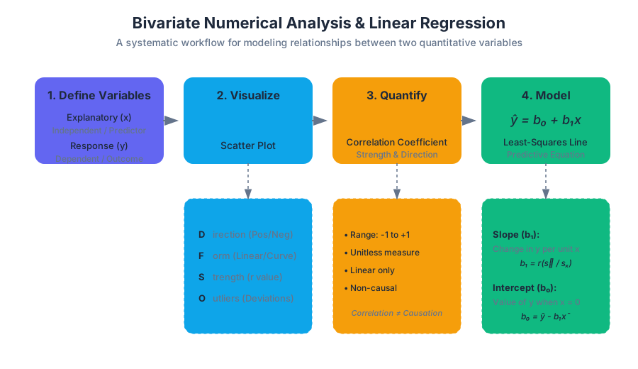
In the realm of statistical modeling, bivariate numerical data represents the first step toward predictive power. While univariate analysis allows us to understand the distribution and central tendency of a single variable, bivariate analysis explores the dynamic relationship between two quantitative variables. We seek to determine if a change in an explanatory variable ($x$)—also known as the independent variable—is associated with a predictable change in a response variable ($y$), or the dependent variable.
This relationship is the foundation of linear regression, a method that allows us to move beyond simple observation into the territory of estimation and forecasting. By quantifying the "link" between variables, we can construct mathematical models that serve as the backbone for everything from algorithmic trading and medical diagnostics to social science research.
1. Scatter Plots: The Visual Foundation
Before performing any calculation, a statistician must visualize the data. The scatter plot is the primary tool for this task. It maps each pair of observations $(x_i, y_i)$ as a point in a two-dimensional Cartesian plane.
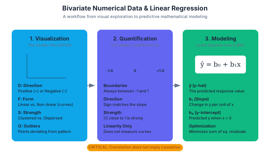
When interpreting a scatter plot, we look for four specific characteristics, often remembered by the acronym DFSO:
- Direction: Is the trend positive (as $x$ increases, $y$ increases) or negative (as $x$ increases, $y$ decreases)?
- Form: Is the relationship linear, or does it follow a curve (quadratic, exponential, logarithmic)?
- Strength: How closely do the points follow the form? Tight clusters indicate a strong relationship; high dispersion indicates a weak one.
- Outliers: Are there individual points that deviate significantly from the overall pattern?
Interpreting Scatter Plot Characteristics
| Characteristic | Description | Visual Indicator |
|---|---|---|
| Positive Association | Both variables move in the same direction. | Points trend from bottom-left to top-right. |
| Negative Association | Variables move in opposite directions. | Points trend from top-left to bottom-right. |
| Linear Form | The rate of change is constant. | Points roughly follow a straight line. |
| Non-linear Form | The rate of change varies. | Points follow a curve, "U" shape, or "S" shape. |
| Strong Strength | High predictive reliability. | Points are very close to the imaginary trend line. |
| Weak Strength | Low predictive reliability. | Points appear as a "cloud" with a vague trend. |
2. The Correlation Coefficient (r)
While scatter plots provide a qualitative "feel" for the data, the Correlation Coefficient ($r$), specifically the Pearson Product-Moment Correlation, provides a quantitative measure of the strength and direction of a linear relationship.
Mathematically, $r$ is the average product of the $z$-scores of the $x$ and $y$ pairs:
$$r = \frac{1}{n-1} \sum \left( \frac{x_i - \bar{x}}{s_x} \right) \left( \frac{y_i - \bar{y}}{s_y} \right)$$
Properties of $r$
- Boundaries: $r$ is always between $-1$ and $1$.
- Direction: $r > 0$ indicates a positive slope; $r < 0$ indicates a negative slope.
- Strength: $|r| = 1$ is a perfect linear relationship; $r = 0$ indicates no linear relationship.
- Unitless: Because it uses $z$-scores, $r$ is not affected by changes in units (e.g., converting inches to centimeters).
- Symmetry: The correlation of $(x, y)$ is the same as the correlation of $(y, x)$.
Critical Insight: Correlation does not imply causation. A high $r$ value simply means the two variables move together; it does not prove that $x$ causes $y$. "Lurking variables" or confounding factors may be the actual drivers of the observed relationship.
3. The Least-Squares Regression Line (LSRL)
If the scatter plot reveals a linear form, we can model the relationship using the Least-Squares Regression Line (LSRL). This is the "line of best fit" that minimizes the sum of the squared vertical distances between the observed data points and the line itself.
The equation for the LSRL is typically written as: $$\hat{y} = b_0 + b_1x$$
Where:
- $\hat{y}$ (y-hat) is the predicted value of $y$ for a given $x$.
- $b_1$ is the slope, representing the predicted change in $y$ for every 1-unit increase in $x$.
- $b_0$ is the y-intercept, representing the predicted value of $y$ when $x = 0$.
Calculating the Parameters
The slope and intercept are derived from the means ($\bar{x}, \bar{y}$), standard deviations ($s_x, s_y$), and the correlation coefficient ($r$):
- Slope ($b_1$): $b_1 = r \left( \frac{s_y}{s_x} \right)$
- Intercept ($b_0$): $b_0 = \bar{y} - b_1\bar{x}$
Mathematical Derivation: The Normal Equations
The goal is to minimize the Loss Function $L = \sum (y_i - (b_0 + b_1x_i))^2$. By taking partial derivatives with respect to $b_0$ and $b_1$ and setting them to zero, we arrive at the "Normal Equations."
\begin{aligned}
\text{1. Partial wrt } b_0: & \quad \frac{\partial}{\partial b_0} \sum (y_i - b_0 - b_1x_i)^2 = -2 \sum (y_i - b_0 - b_1x_i) = 0 \\
\text{2. Partial wrt } b_1: & \quad \frac{\partial}{\partial b_1} \sum (y_i - b_0 - b_1x_i)^2 = -2 \sum x_i(y_i - b_0 - b_1x_i) = 0 \\
\\
\text{Resulting in:} & \\
n b_0 + b_1 \sum x_i &= \sum y_i \\
b_0 \sum x_i + b_1 \sum x_i^2 &= \sum x_i y_i
\end{aligned}
4. Residuals and Residual Plots
No model is perfect. The difference between an observed value ($y$) and the predicted value ($\hat{y}$) is called a residual.
$$\text{Residual} = y - \hat{y}$$
- A positive residual means the observed value was higher than predicted (the model underestimated).
- A negative residual means the observed value was lower than predicted (the model overestimated).
The Residual Plot
To validate a linear model, we plot the residuals on the vertical axis against the explanatory variable ($x$) on the horizontal axis.
- If the residual plot shows a random scatter of points around the horizontal line at 0, the linear model is appropriate.
- If the residual plot shows a clear pattern (like a curve), a non-linear model may be better suited for the data.
- If the "spread" of residuals increases or decreases as $x$ increases (heteroscedasticity), the reliability of our predictions varies across the range of $x$.
| Residual Plot Appearance | Interpretation |
|---|---|
| Uniform Random Scatter | Linear model is appropriate; constant variance. |
| Curved Pattern (U-shape) | Relationship is likely non-linear; use transformation. |
| Fan/Funnel Shape | Heteroscedasticity; prediction error grows with $x$. |
| Isolated Outliers | Specific data points exert undue influence or are errors. |
5. The Coefficient of Determination ($r^2$)
While $r$ tells us about direction and strength, $r^2$ (r-squared) tells us about the proportion of variability. It is formally defined as the percentage of the variation in the response variable ($y$) that can be explained by the linear relationship with the explanatory variable ($x$).
$$r^2 = \frac{\text{SST} - \text{SSE}}{\text{SST}} = \frac{\text{SSR}}{\text{SST}}$$
Where:
- SST (Total Sum of Squares): Total variation in $y$.
- SSE (Sum of Squared Errors): Variation not explained by the line (sum of squared residuals).
- SSR (Regression Sum of Squares): Variation explained by the line.
Example Interpretation: If $r^2 = 0.85$ for a model relating "Study Hours" to "Exam Scores," we say: "85% of the variation in exam scores can be explained by the linear relationship with study hours. The remaining 15% is due to other factors or inherent variability."
6. Influential Points and Outliers
Not all data points are created equal. In bivariate data, we distinguish between different types of unusual observations:
- Outliers: Points with large residuals (they don't fit the $y$-pattern).
- High Leverage Points: Points with $x$-values that are far from the mean of $x$. They have the potential to "pull" the regression line toward themselves.
- Influential Points: A point is influential if removing it significantly changes the slope, intercept, or $r$ value of the regression. Most influential points have high leverage.
Comparison of Point Types
| Point Type | Location | Effect on Residual | Effect on LSRL |
|---|---|---|---|
| Vertical Outlier | Far from the line in $y$-direction. | Large residual. | Usually minimal effect on slope. |
| High Leverage | Far from the mean in $x$-direction. | Can be small or large. | Acts as a "pivot" for the line. |
| Influential | High leverage + Outlier. | Variable. | Drastically changes the slope ($b_1$). |
7. Pitfalls: Extrapolation and Lurking Variables
Even a perfect model has limits. Two major traps await the unwary analyst:
Extrapolation
Extrapolation is the practice of using a regression line to predict values outside the range of the observed $x$-data. Example: If you track a child's growth from ages 2 to 10, the linear model might predict they will be 12 feet tall by age 30. Linear trends rarely continue indefinitely; the relationship may change or level off outside the observed domain.
Lurking Variables and Confounding
A lurking variable is a variable that is not included in the study but has an effect on the variables of interest. Example: There is a strong positive correlation between ice cream sales and drowning incidents. However, ice cream does not cause drowning. The lurking variable is Temperature—hot weather increases both ice cream consumption and the number of people swimming.
Source Materials
Study Statistics and Probability on Lykke
This course page is free to open: signed out, you can read its first two sections, and signing in, on any plan, opens the rest. The free Lykke Chrome extension syncs your own Canvas courses, so ChatGPT, Claude and Muse can answer from your classes and deadlines. It only reads Canvas.
Add the free extensionSign in to open every sectionAll sections of Statistics and Probability · Browse more course pages