From the free course Spring 2026 - Math 354 - Sections 02/04 on Lykke
The Simplex Method and Tableau Optimization
Key concepts: Simplex Tableau · Pivot Selection · Optimality Criterion · Entering and Leaving Variables · Iterative Improvement
The primary algorithmic approach for solving linear programming problems using iterative pivoting.
The Simplex Method and Tableau Optimization
The Simplex Method is arguably the most influential algorithm in the history of constrained optimization. Developed by George Dantzig in 1947, it provides a systematic, iterative procedure for navigating the vertices of a high-dimensional polytope to find the optimal value of a linear objective function. While modern interior-point methods offer better theoretical polynomial time complexity, the Simplex algorithm remains the workhorse of industrial solvers due to its efficiency in practice and its unique ability to perform "warm starts" after minor model modifications.
At its core, the Simplex method exploits a fundamental property of Linear Programming (LP): if an optimal solution exists, it must occur at an extreme point (vertex) of the feasible region. Instead of searching the infinite interior of the feasible set, the algorithm "hops" from one vertex to an adjacent one, ensuring that each move improves (or at least maintains) the value of the objective function.
Foundations: Standard and Canonical Forms
Before the Simplex method can be applied, a Linear Programming problem must be expressed in a specific mathematical structure. In academic and professional practice, we distinguish between Standard Form and Canonical Form.
Standard Form
A maximization problem is in Standard Form if:
- The objective function is to be maximized.
- All variables are non-negative ($x_i \ge 0$).
- All constraints are expressed as "less-than-or-equal-to" inequalities ($\sum a_{ij}x_j \le b_i$).
- All right-hand side constants are non-negative ($b_i \ge 0$).
Canonical Form
To perform the algebraic manipulations required by the Simplex method, we must convert inequalities into equalities. This is achieved by introducing Slack Variables. A problem is in Canonical Form if it consists of a system of linear equations $Ax = b$ where a subset of the columns of $A$ forms an identity matrix.
Definition: Slack Variable A non-negative variable $s_i$ added to a $\le$ constraint to convert it into an equality. For example, $2x + 3y \le 6$ becomes $2x + 3y + s_1 = 6$, where $s_1 \ge 0$.
| Feature | Standard Form | Canonical Form |
|---|---|---|
| Constraint Type | Inequalities ($\le$) | Equalities ($=$) |
| Variable Count | Original decision variables | Decision + Slack/Artificial variables |
| Goal | Geometric definition of the polytope | Algebraic setup for Gauss-Jordan elimination |
| RHS ($b$) | Must be non-negative | Must be non-negative |
The Simplex Tableau
The Simplex Tableau is a structured matrix used to organize the coefficients of the objective function and the constraints. It serves as a computational "dashboard" that tracks the current Basic Feasible Solution (BFS).
In any iteration, the variables are partitioned into two sets:
- Basic Variables (BV): Variables that currently form the basis (the identity matrix columns). Their values are determined by the right-hand side.
- Non-Basic Variables (NBV): Variables set to zero.
Tableau Anatomy
A typical maximization tableau is organized as follows:
- The top row (often called the z-row) contains the coefficients of the objective function.
- The remaining rows represent the constraints.
- The last column (RHS) contains the current values of the basic variables.
The Simplex Algorithm: Iterative Improvement
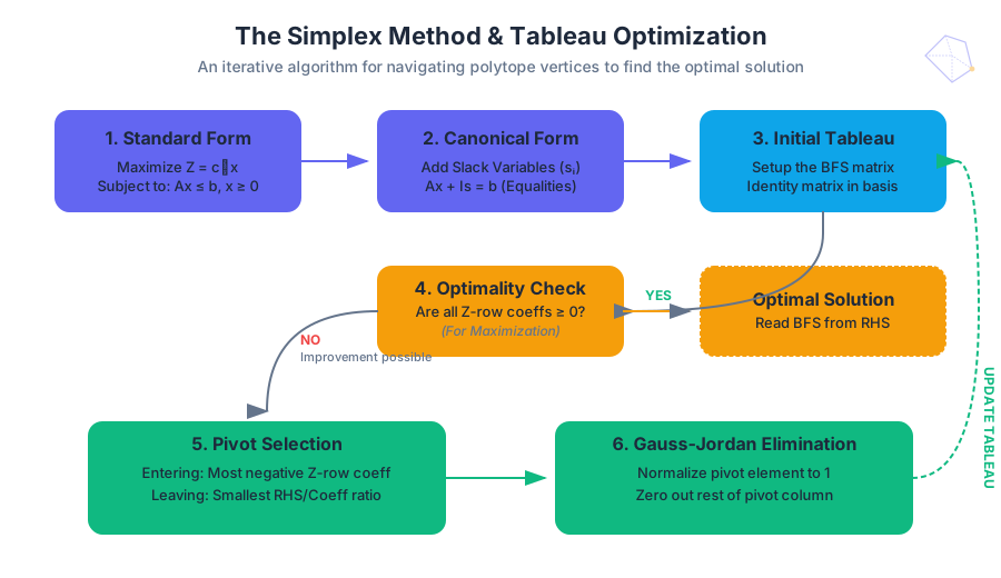
The algorithm follows a rigorous cycle of selection and transformation. Each iteration represents a move from one vertex to an adjacent vertex with a better objective value.
1. Optimality Criterion
We examine the objective row (z-row). In a maximization problem, if all coefficients of the non-basic variables in the z-row are non-negative (assuming the form $z - \sum c_i x_i = 0$), the current solution is optimal. If any coefficients are negative, the objective can still be improved.
2. Pivot Selection: The Entering Variable
The non-basic variable with the most negative coefficient in the z-row is chosen as the Entering Variable. This variable will transition from zero to a positive value in the next iteration. This choice is a heuristic known as "Dantzig's Rule," aimed at increasing the objective function as steeply as possible.
3. The Minimum Ratio Test: The Leaving Variable
To maintain feasibility, we cannot increase the entering variable indefinitely. We must determine which basic variable hits zero first. For every row where the entering variable has a positive coefficient, we calculate the ratio: $$\text{Ratio} = \frac{\text{RHS Value}}{\text{Coefficient of Entering Variable}}$$ The row with the smallest non-negative ratio identifies the Leaving Variable. This row is called the Pivot Row.
4. Pivoting (Gauss-Jordan Elimination)
The intersection of the entering column and the leaving row is the Pivot Element. We perform row operations to:
- Turn the pivot element into a $1$.
- Turn all other elements in the entering column (including the z-row) into $0$.
Implementation: Low-Level Pivot Logic
The following Python implementation using NumPy demonstrates the core mechanics of a single Simplex iteration. Note the use of the minimum ratio test and row-wise transformations.
import numpy as np

def simplex_step(tableau):
    """
    Performs a single pivot iteration on a Simplex Tableau.
    Assumes maximization problem in the form: z - c1x1 - c2x2 ... = 0
    """
    n_rows, n_cols = tableau.shape
    z_row = tableau[0, :-1]

    # 1. Check Optimality / Select Entering Variable (Pivot Column)
    if np.all(z_row >= 0):
        return None, "Optimal"

    pivot_col = np.argmin(z_row)

    # 2. Minimum Ratio Test / Select Leaving Variable (Pivot Row)
    ratios = []
    for i in range(1, n_rows):
        val = tableau[i, pivot_col]
        rhs = tableau[i, -1]
        if val > 0:
            ratios.append(rhs / val)
        else:
            ratios.append(np.inf) # Cannot pivot on non-positive elements

    pivot_row = np.argmin(ratios) + 1 # +1 because we skipped z-row

    if ratios[pivot_row-1] == np.inf:
        return None, "Unbounded"

    # 3. Pivoting
    pivot_val = tableau[pivot_row, pivot_col]
    tableau[pivot_row, :] /= pivot_val

    for r in range(n_rows):
        if r != pivot_row:
            tableau[r, :] -= tableau[r, pivot_col] * tableau[pivot_row, :]

    return tableau, "Iterating"

# Example usage:
# Maximize z = 3x1 + 2x2 subject to 2x1 + x2 <= 4, 2x1 + 3x2 <= 6
# Tableau: [z, x1, x2, s1, s2, RHS]
example_tab = np.array([
    [1, -3, -2, 0, 0, 0],
    [0,  2,  1, 1, 0, 4],
    [0,  2,  3, 0, 1, 6]
], dtype=float)

new_tab, status = simplex_step(example_tab)
print(f"Status: {status}\nUpdated Tableau:\n{new_tab}")
Mathematical Derivation of the Pivot
To understand why the Simplex method works, we must look at the linear algebra of the basis. Let the constraints be $Ax = b$. We partition $A$ into $[B, N]$, where $B$ is the basis matrix (invertible) and $N$ represents non-basic columns.
The solution is given by: $$x_B = B^{-1}b - B^{-1}Nx_N$$ The objective function $z = c^T x$ becomes: $$z = c_B^T(B^{-1}b - B^{-1}Nx_N) + c_N^T x_N$$ $$z = c_B^T B^{-1}b + (c_N^T - c_B^T B^{-1}N)x_N$$
The term $(c_N^T - c_B^T B^{-1}N)$ is known as the Reduced Cost vector. If all reduced costs are non-positive (for maximization), then increasing any $x_N$ (which are currently 0) will decrease $z$. Thus, we are at the optimum.
\begin{aligned}
&\text{Algorithm: Simplex Method}\\
&\text{1: Identify initial BFS by setting } x_{non-basic} = 0 \\
&\text{2: } \mathbf{while} \ \exists \ \bar{c}_j < 0 \ \mathbf{do} \\
&\text{3: } \quad \text{Select } j \text{ such that } \bar{c}_j \text{ is most negative (Entering Variable)} \\
&\text{4: } \quad \mathbf{if} \ A_{ij} \le 0 \ \forall i \ \mathbf{then} \\
&\text{5: } \quad \quad \mathbf{return} \ \text{"Unbounded"} \\
&\text{6: } \quad \text{Select row } i \text{ such that } \frac{b_i}{A_{ij}} = \min_{k: A_{kj}>0} \frac{b_k}{A_{kj}} \text{ (Leaving Variable)} \\
&\text{7: } \quad \text{Perform pivot on } A_{ij} \text{ using Gauss-Jordan elimination} \\
&\text{8: } \mathbf{end \ while} \\
&\text{9: } \mathbf{return} \ \text{Current BFS}
\end{aligned}
Worked Example: Maximizing a Three-Variable System
Consider the following problem from Participation #4: Maximize: $z = 4x_1 + 2x_2 + 7x_3$ Subject to:
- $2x_1 - x_2 + 4x_3 \le 18$
- $4x_1 + 2x_2 + 5x_3 \le 10$
- $x_1, x_2, x_3 \ge 0$
Step 1: Convert to Canonical Form
Introduce slack variables $s_1, s_2$:
- $2x_1 - x_2 + 4x_3 + s_1 = 18$
- $4x_1 + 2x_2 + 5x_3 + s_2 = 10$ Objective: $z - 4x_1 - 2x_2 - 7x_3 = 0$
Step 2: Initial Tableau
| Basis | $z$ | $x_1$ | $x_2$ | $x_3$ | $s_1$ | $s_2$ | RHS |
|---|---|---|---|---|---|---|---|
| $z$ | 1 | -4 | -2 | -7 | 0 | 0 | 0 |
| $s_1$ | 0 | 2 | -1 | 4 | 1 | 0 | 18 |
| $s_2$ | 0 | 4 | 2 | 5 | 0 | 1 | 10 |
Step 3: First Pivot
- Entering: $x_3$ (most negative in z-row: -7).
- Ratios:
- Row 1 ($s_1$): $18 / 4 = 4.5$
- Row 2 ($s_2$): $10 / 5 = 2$
- Leaving: $s_2$ (smallest ratio).
- Pivot Element: 5 (Row 2, Column $x_3$).
After pivoting on 5:
- Divide Row 2 by 5.
- $R_1 \leftarrow R_1 - 4R_2$
- $R_z \leftarrow R_z + 7R_2$
New Tableau:
| Basis | $z$ | $x_1$ | $x_2$ | $x_3$ | $s_1$ | $s_2$ | RHS |
|---|---|---|---|---|---|---|---|
| $z$ | 1 | 1.6 | 0.8 | 0 | 0 | 1.4 | 14 |
| $s_1$ | 0 | -1.2 | -2.6 | 0 | 1 | -0.8 | 10 |
| $x_3$ | 0 | 0.8 | 0.4 | 1 | 0 | 0.2 | 2 |
Result: All coefficients in the z-row are non-negative ($1.6, 0.8, 0, 0, 1.4$). The solution is optimal. Optimal Solution: $x_1=0, x_2=0, x_3=2, z=14$.
Advanced Scenarios and Pitfalls
While the Simplex method is robust, several edge cases can occur during the execution of the algorithm.
1. Degeneracy and Cycling
Degeneracy occurs when one or more basic variables have a value of zero. This happens when there is a tie in the Minimum Ratio Test.
- The Risk: The algorithm might pivot without changing the objective value. In rare cases, it can enter an infinite loop (cycling).
- The Solution: Use Bland’s Rule, which dictates choosing the variable with the lowest index in case of ties.
2. Unboundedness
If the entering variable has no positive coefficients in any constraint row, the ratio test fails.
- Meaning: The feasible region is open in the direction of improvement. The objective function can be increased to infinity.
3. Infeasibility and the Two-Phase Method
If the origin $(0,0,...0)$ is not a feasible solution (e.g., if we have $\ge$ constraints), we cannot start the Simplex method directly.
- Phase I: Introduce Artificial Variables and a new objective function to minimize the sum of these variables. If the minimum is 0, we have found a BFS for the original problem.
- Phase II: Remove artificial variables and solve the original objective.
| Problem State | Tableau Indicator |
|---|---|
| Optimal | All z-row coefficients $\ge 0$ (Max problem). |
| Unbounded | Entering column has all entries $\le 0$. |
| Infeasible | Phase I ends with a non-zero artificial variable. |
| Multiple Optima | A non-basic variable has a 0 coefficient in the optimal z-row. |
Real-World Usage: Large-Scale Solvers
In production environments, we rarely write our own Simplex solvers from scratch. Instead, we use high-performance libraries like Gurobi, CPLEX, or the open-source HiGHS. These solvers use the Revised Simplex Method, which maintains the basis inverse $B^{-1}$ explicitly or via LU factorization to save memory and computation time.
# Example: Solving an LP using the GLPK (GNU Linear Programming Kit)
# 1. Define the problem in a .mod or .lp file
cat <<EOF > problem.lp
Maximize
 obj: 4 x1 + 2 x2 + 7 x3
Subject To
 c1: 2 x1 - 1 x2 + 4 x3 <= 18
 c2: 4 x1 + 2 x2 + 5 x3 <= 10
Bounds
 x1 >= 0
 x2 >= 0
 x3 >= 0
End
EOF

# 2. Run the solver using the Simplex method
glpsol --lp problem.lp -o solution.txt

# 3. View the results
grep "Objective:" solution.txt
Summary of Key Insights
- Geometric Intuition: The Simplex method is a "greedy" walk along the edges of a polytope.
- Algebraic Engine: The tableau is a compact representation of Gauss-Jordan elimination tailored for optimization.
- The Ratio Test: This is the "safety valve" that prevents the algorithm from stepping outside the feasible region.
- Duality: Every Simplex step in the primal problem implicitly provides information about the dual problem (shadow prices), which are represented by the coefficients in the optimal z-row.
By mastering the tableau and the logic of pivots, one gains the ability to not only solve linear programs but to perform sensitivity analysis—understanding how changes in constraints or costs ripple through a complex system.
Source Materials
Study Spring 2026 - Math 354 - Sections 02/04 on Lykke
This course page is free to open: signed out, you can read its first two sections, and signing in, on any plan, opens the rest. The free Lykke Chrome extension syncs your own Canvas courses, so ChatGPT, Claude and Muse can answer from your classes and deadlines. It only reads Canvas.
Add the free extensionSign in to open every sectionAll sections of Spring 2026 - Math 354 - Sections 02/04 · Browse more course pages