From the free course Spring 2026 - Math 354 - Sections 02/04 on Lykke
Graphical Optimization and the Geometric Method
Key concepts: Feasible Region · Extreme Point Theorem · Level Curves · Vertices · Boundedness
Solving 2D linear programming problems using geometric visualization, feasible regions, and level curves.
Graphical Optimization and the Geometric Method
In the study of Linear Programming (LP), the Geometric Method serves as the foundational bridge between abstract algebraic constraints and spatial intuition. While modern industrial solvers handle problems with millions of variables using the Simplex method or Interior Point methods, the core logic of these algorithms is rooted in the geometry of two and three dimensions.
For problems involving only two decision variables, we can visualize the entire optimization landscape. This visualization reveals the "why" behind the "how"—explaining why optimal solutions naturally gravitate toward the "corners" of the search space and how the objective function "scans" the feasible region to find the best possible outcome.
The Anatomy of a Linear Program
Before applying geometric techniques, we must understand the structure of the problem. A linear program consists of an objective function to be maximized or minimized, subject to a set of linear constraints and non-negativity requirements.
Standard vs. Canonical Form
In mathematical optimization, the representation of the problem dictates the method of solution.
- Standard Form: Typically characterized by a maximization objective, all constraints expressed as "less-than-or-equal-to" ($\le$) inequalities, and all variables restricted to non-negative values.
- Canonical Form: Characterized by equality constraints ($Ax = b$), achieved by introducing slack variables to "soak up" the difference between the left and right sides of an inequality.
| Feature | Standard Form | Canonical Form |
|---|---|---|
| Objective | Maximize $z = \mathbf{c}^T\mathbf{x}$ | Maximize $z = \mathbf{c}^T\mathbf{x}$ |
| Constraints | $A\mathbf{x} \le \mathbf{b}$ | $A\mathbf{x} = \mathbf{b}$ |
| Variables | $\mathbf{x} \ge 0$ | $\mathbf{x} \ge 0$ (including slacks) |
| Geometric View | Intersection of half-planes | Intersection of hyperplanes and orthants |
| Primary Use | Graphical Method / Initial Setup | Simplex Method / Matrix Algebra |
The Feasible Region: Geometry of Constraints
The Feasible Region (often denoted as $\mathcal{F}$) is the set of all points $(x, y)$ that satisfy every constraint in the system simultaneously.
Mathematical Definition
Mathematically, each linear inequality of the form $ax + by \le c$ defines a half-plane in $\mathbb{R}^2$. The feasible region is the intersection of these half-planes.
Definition: Convexity A set $\mathcal{F}$ is convex if, for any two points $P_1, P_2 \in \mathcal{F}$, the entire line segment connecting $P_1$ and $P_2$ also lies within $\mathcal{F}$.
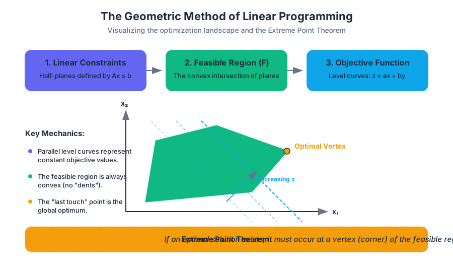
In Linear Programming, the feasible region is always a convex polytope (a polygon in 2D, a polyhedron in 3D). This property is critical because it ensures that there are no "local" optima that are not also "global" optima. If you find a peak in a convex region, it is the only peak.
Constructing the Region
- Treat inequalities as equations: Graph the lines $ax + by = c$.
- Identify the valid side: Use a test point (usually $(0,0)$) to determine which side of the line satisfies the inequality.
- Find the intersection: The region where all shaded areas overlap is the feasible region.
- Apply non-negativity: Restrict the region to the first quadrant ($x \ge 0, y \ge 0$).
Level Curves and the Objective Function
The objective function $z = f(x, y) = ax + by$ defines a surface in three-dimensional space. However, in the geometric method, we project this onto the 2D plane using Level Curves (also known as isoclines or objective lines).
Mechanics of Level Curves
A level curve represents all points $(x, y)$ that yield the same value for $z$. For example, if $z = 2x + 3y$, the level curve for $z=6$ is the line $2x + 3y = 6$.
As we change the value of $z$, the level curve shifts across the plane. Crucially, all level curves for a linear objective function are parallel to each other. Their slope is determined by the ratio of the coefficients of the decision variables: $m = -a/b$.
The Optimization "Scan"
To solve the problem graphically:
- Draw a "base" level curve for an arbitrary value of $z$ (e.g., $z=0$).
- Move this line in the direction of increasing $z$ (for maximization) or decreasing $z$ (for minimization).
- The last point in the feasible region that the level curve touches before exiting the region is the optimal solution.
The Extreme Point Theorem
Why do we only look at the corners? This is answered by the Extreme Point Theorem (or the Fundamental Theorem of Linear Programming).
Theorem: Extreme Point Theorem If a linear programming problem has an optimal solution, then at least one optimal solution occurs at an extreme point (vertex) of the feasible region.
Derivation and Logic
Consider the feasible region $\mathcal{F}$. If the optimal solution were in the interior of $\mathcal{F}$, we could move a small distance in the direction of the objective function's gradient to increase $z$, meaning the interior point could not have been optimal. Therefore, the optimum must lie on the boundary.
If the optimum lies on a boundary line segment but not at a vertex, then every point on that segment yields the same $z$ value. This implies that the vertices at the ends of that segment are also optimal. Thus, we are mathematically justified in only checking the vertices.
| Element | Geometric Description | Algebraic Description |
|---|---|---|
| Vertex | A "corner" where two or more boundary lines intersect. | A Basic Feasible Solution (BFS). |
| Edge | A line segment connecting two adjacent vertices. | A path where one constraint is tight and others vary. |
| Interior | Points not on any constraint boundary. | Solutions where all slack variables are non-zero. |
Worked Example: Maximization with Multiple Constraints
Consider the following problem from Participation #2: Maximize $z = 2x + 3y$ Subject to:
- $x + 3y \le 9$
- $2x + 3y \le 12$
- $x \ge 0, y \ge 0$
Step 1: Find the Vertices
We find the vertices by solving the systems of equations formed by the intersection of the boundary lines.
- Origin: $(0, 0)$
- Y-intercept of (1): Set $x=0$ in $x + 3y = 9 \implies y=3$. Point: $(0, 3)$.
- X-intercept of (2): Set $y=0$ in $2x + 3y = 12 \implies x=6$. Point: $(6, 0)$.
- Intersection of (1) and (2): Subtract (1) from (2): $(2x + 3y) - (x + 3y) = 12 - 9 \implies x = 3$. Substitute $x=3$ into (1): $3 + 3y = 9 \implies 3y = 6 \implies y = 2$. Point: $(3, 2)$.
Step 2: Evaluate the Objective Function
We test each vertex in the objective function $z = 2x + 3y$.
| Vertex $(x, y)$ | $z = 2x + 3y$ | Status |
|---|---|---|
| $(0, 0)$ | $2(0) + 3(0) = 0$ | Minimum |
| $(0, 3)$ | $2(0) + 3(3) = 9$ | |
| $(6, 0)$ | $2(6) + 3(0) = 12$ | |
| $(3, 2)$ | $2(3) + 3(2) = 12$ | Optimal (Tie) |
Note: In this specific case, both $(6,0)$ and $(3,2)$ yield $z=12$. This indicates that the objective function line is parallel to the constraint line $2x + 3y = 12$. Every point on the segment connecting these two vertices is optimal.
Implementation: Computational Geometry
While we visualize in 2D, we often use libraries to solve these problems. Below is a Python implementation using SciPy to solve the example above, followed by a low-level conceptual look at how we might verify a vertex's feasibility in C.
import numpy as np
from scipy.optimize import linprog

# Objective: Maximize z = 2x + 3y
# Note: linprog only minimizes, so we minimize -z = -2x - 3y
c = [-2, -3]

# Inequality constraints matrix A_ub * x <= b_ub
# x + 3y <= 9
# 2x + 3y <= 12
A = [[1, 3],
     [2, 3]]
b = [9, 12]

# Bounds for x and y (non-negativity)
x_bounds = (0, None)
y_bounds = (0, None)

res = linprog(c, A_ub=A, b_ub=b, bounds=[x_bounds, y_bounds], method='highs')

print(f"Optimal Value: {-res.fun}")
print(f"Coordinates: x={res.x[0]}, y={res.x[1]}")
The mathematical transformation from an inequality to a canonical equality (Participation #3) is the precursor to the Simplex algorithm.
\begin{aligned}
&\text{Maximize } z = 4x_1 + 2x_2 + 7x_3 \\
&\text{Subject to:} \\
&2x_1 - x_2 + 4x_3 + s_1 = 18 \\
&4x_1 + 2x_2 + 5x_3 + s_2 = 10 \\
&x_1, x_2, x_3, s_1, s_2 \ge 0
\end{aligned}
In a systems-level context, checking if a point is a "vertex" involves verifying linear independence of the active constraints.
#include <stdio.h>
#include <stdbool.h>

/**
 * Simple check to see if a point (x, y) violates any constraints.
 * In a real engine, this would use an epsilon for floating point comparison.
 */
bool is_feasible(float x, float y, float A[2][2], float b[2]) {
    if (x < 0 || y < 0) return false;

    for (int i = 0; i < 2; i++) {
        if ((A[i][0] * x + A[i][1] * y) > b[i] + 0.0001f) {
            return false;
        }
    }
    return true;
}

int main() {
    float A[2][2] = {{1, 3}, {2, 3}};
    float b[2] = {9, 12};

    float test_x = 3.0, test_y = 2.0;

    if (is_feasible(test_x, test_y, A, b)) {
        printf("Point (%.2f, %.2f) is feasible.\n", test_x, test_y);
    } else {
        printf("Point (%.2f, %.2f) violates constraints.\n", test_x, test_y);
    }

    return 0;
}
Boundedness and Special Cases
Not every linear program results in a neat, single-point solution. The geometry of the problem can lead to four distinct outcomes.
| Outcome | Geometric Description | Practical Meaning |
|---|---|---|
| Unique Optimal | The level curve hits exactly one vertex last. | One clear best strategy. |
| Alternative Optima | The level curve is parallel to a constraint edge. | Multiple strategies yield the same best result. |
| Unbounded | The feasible region is "open" in the direction of improvement. | The model is missing a constraint; profit is infinite. |
| Infeasible | The constraints do not overlap; no feasible region exists. | The requirements are contradictory (e.g., $x \le 2$ and $x \ge 5$). |
Unboundedness
An unbounded solution occurs when the feasible region extends infinitely in a direction that allows the objective function to increase (or decrease) without limit. In the real world, this usually indicates a flawed model—no physical system allows for infinite profit or zero cost with infinite production.
Infeasibility
Infeasibility is often encountered in complex projects where resources are over-constrained. Geometrically, this means the intersection of the half-planes is the empty set.
From 2D Geometry to N-Dimensional Algebra
The Graphical Method is limited to 2 or 3 variables because humans cannot visualize higher-dimensional polytopes (hyper-polyhedra). However, the logic holds:
- In $N$ dimensions, a constraint is a hyperplane.
- The feasible region is a convex simplex.
- The optimal solution is still at a vertex.
The Simplex Method is essentially an algebraic "walk" along the edges of this high-dimensional shape. It starts at one vertex (usually the origin) and moves to an adjacent vertex that improves the objective function value, continuing until no further improvement is possible.
Source Materials
Study Spring 2026 - Math 354 - Sections 02/04 on Lykke
This course page is free to open: signed out, you can read its first two sections, and signing in, on any plan, opens the rest. The free Lykke Chrome extension syncs your own Canvas courses, so ChatGPT, Claude and Muse can answer from your classes and deadlines. It only reads Canvas.
Add the free extensionSign in to open every sectionAll sections of Spring 2026 - Math 354 - Sections 02/04 · Browse more course pages