From the free course Spring 2026 - Math 354 - Sections 02/04 on Lykke
Duality in Linear Programming
Key concepts: Primal Problem · Dual Problem · Weak Duality Theorem · Duality Theorem · Shadow Prices
Exploring the relationship between a 'Primal' problem and its 'Dual' counterpart.
Duality in Linear Programming: The Hidden Symmetry of Optimization
In the realm of mathematical optimization, Duality is perhaps the most profound and elegant concept. It suggests that every linear programming (LP) problem, referred to as the Primal, can be viewed from an entirely different perspective, known as the Dual. This is not merely a mathematical curiosity; the relationship between these two problems provides deep insights into the structure of optimization, the value of resources, and the stability of optimal solutions.
As we explore this topic, we will see that the Dual problem is essentially the "mirror image" of the Primal. If the Primal is a maximization of profit subject to resource constraints, the Dual is the minimization of the total value of those resources. This symmetry allows us to solve complex problems more efficiently and perform Sensitivity Analysis—determining how changes in our constraints (like a sudden shortage of raw materials) affect our bottom line.
The Primal and Dual Relationship
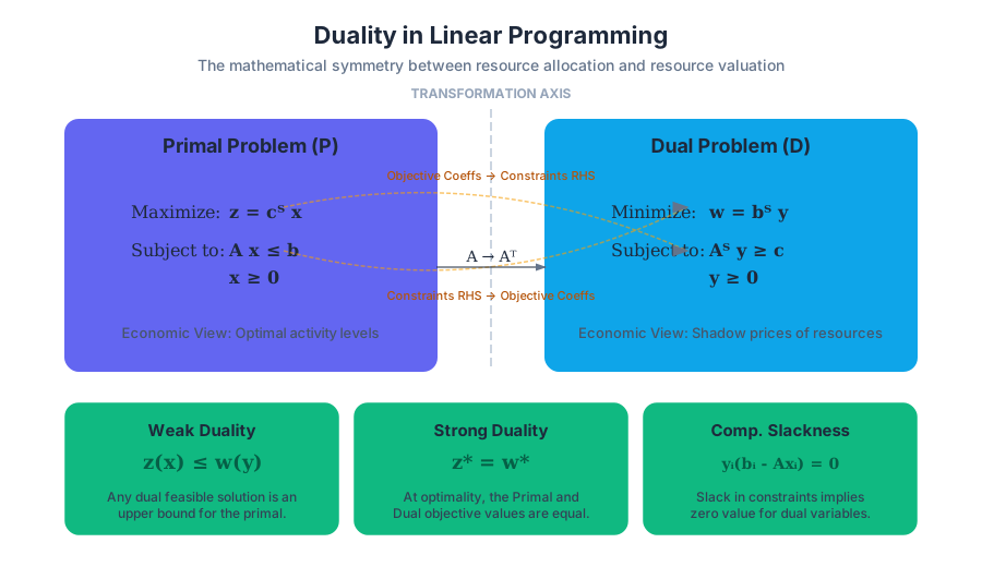
To understand duality, we must first establish a standard frame of reference. In linear programming, we often work with the Standard Form or Canonical Form. A Primal problem in maximization form is typically defined by an objective function $z = \mathbf{c}^T\mathbf{x}$, subject to a set of linear inequalities $A\mathbf{x} \le \mathbf{b}$ and non-negativity constraints $\mathbf{x} \ge 0$.
The Dual Problem is constructed using the same parameters ($A, \mathbf{b}, \mathbf{c}$) but rearranged. The coefficients of the Primal objective function become the right-hand side (RHS) of the Dual constraints, and the Primal RHS values become the coefficients of the Dual objective function.
Construction Rules
The transformation from Primal to Dual follows a strict set of mapping rules. These rules ensure that the mathematical integrity of the optimization is preserved across the "mirror."
| Primal Feature (Maximization) | Dual Feature (Minimization) |
|---|---|
| Objective Function $z = \sum c_j x_j$ | Objective Function $w = \sum b_i y_i$ |
| Constraint $i$: $\sum a_{ij} x_j \le b_i$ | Variable $y_i$: $y_i \ge 0$ |
| Constraint $i$: $\sum a_{ij} x_j = b_i$ | Variable $y_i$: $y_i$ is unrestricted (URS) |
| Variable $x_j$: $x_j \ge 0$ | Constraint $j$: $\sum a_{ij} y_i \ge c_j$ |
| Variable $x_j$: $x_j$ is unrestricted (URS) | Constraint $j$: $\sum a_{ij} y_i = c_j$ |
| Constraint Matrix: $A$ | Constraint Matrix: $A^T$ (Transpose) |
Mathematical Derivation
Consider the Primal problem (P): $$\text{Maximize } z = \mathbf{c}^T\mathbf{x}$$ $$\text{subject to } A\mathbf{x} \le \mathbf{b}, \mathbf{x} \ge 0$$
The Dual problem (D) is formulated as: $$\text{Minimize } w = \mathbf{b}^T\mathbf{y}$$ $$\text{subject to } A^T\mathbf{y} \ge \mathbf{c}, \mathbf{y} \ge 0$$
Where:
- $\mathbf{x}$ is a vector of $n$ decision variables.
- $\mathbf{y}$ is a vector of $m$ dual variables (one for each Primal constraint).
- $A$ is an $m \times n$ matrix of coefficients.
Theorem: The Dual of the Dual is the Primal. If you take the Dual of a Dual problem, you will arrive back at the original Primal problem. This confirms the perfectly symmetric nature of the relationship.
The Fundamental Theorems of Duality
The relationship between the Primal and Dual is governed by three critical theorems. These theorems provide the "guarantees" that allow us to use the Dual to solve or verify the Primal.
1. Weak Duality Theorem
The Weak Duality Theorem states that for any feasible solution $\mathbf{x}$ to the Primal and any feasible solution $\mathbf{y}$ to the Dual: $$\mathbf{c}^T\mathbf{x} \le \mathbf{b}^T\mathbf{y}$$
In plain English: any feasible value of the Dual objective function serves as an upper bound for the Primal objective function (in a maximization problem). Conversely, the Primal provides a lower bound for the Dual.
2. Strong Duality Theorem
The Strong Duality Theorem is the cornerstone of LP. It states that if the Primal has an optimal solution $\mathbf{x}^$, then the Dual also has an optimal solution $\mathbf{y}^$, and their objective values are equal: $$z^* = \mathbf{c}^T\mathbf{x}^* = \mathbf{b}^T\mathbf{y}^* = w^*$$
This equality is what allows us to solve the Dual to find the optimal value of the Primal. In many computational scenarios, the Dual might be easier to solve (e.g., if it has fewer constraints than the Primal).
3. Complementary Slackness Theorem
This theorem describes the relationship between the slack variables of one problem and the decision variables of the other. It states that for optimal solutions $\mathbf{x}^$ and $\mathbf{y}^$:
- If a Primal constraint is "slack" (the inequality is not an equality at the optimum), the corresponding Dual variable must be zero.
- If a Primal variable is positive, the corresponding Dual constraint must be "tight" (the inequality holds as an equality).
| Condition | Mathematical Implication |
|---|---|
| $y_i^* > 0$ | $\sum a_{ij} x_j^* = b_i$ (Constraint $i$ is binding) |
| $\sum a_{ij} x_j^* < b_i$ | $y_i^* = 0$ (Resource $i$ is not fully used; its marginal value is zero) |
| $x_j^* > 0$ | $\sum a_{ij} y_i^* = c_j$ (Dual constraint $j$ is binding) |
| $\sum a_{ij} y_i^* > c_j$ | $x_j^* = 0$ (Activity $j$ is too expensive; it is not performed) |
Shadow Prices and Economic Interpretation
One of the most practical applications of duality is the concept of Shadow Prices. In an economic context, if the Primal problem represents maximizing profit from resources, the Dual variables $y_i$ represent the marginal value of those resources.
Definition: Shadow Price The shadow price of a constraint is the amount by which the optimal value of the objective function ($z^*$) would increase if the right-hand side of that constraint ($b_i$) were increased by one unit, assuming the current optimal basis remains the same.
Why Shadow Prices Matter
Imagine a factory that uses labor and electricity to produce goods. If the shadow price of labor is $15, it means that if the factory could acquire one more hour of labor, its total profit would increase by $15. If the market rate for labor is $10/hour, the factory should hire more workers. If the market rate is $20/hour, it should not.
Table: Primal vs. Dual Economic Logic
| Component | Primal Interpretation (Production) | Dual Interpretation (Valuation) |
|---|---|---|
| Variables | Levels of activities (e.g., units to produce) | Unit value of resources (Shadow prices) |
| Objective | Maximize total profit | Minimize total implicit value of resources |
| Constraints | Resource availability limits | Minimum "worth" of resources used in an activity |
| RHS ($b_i$) | Capacity of resource $i$ | Contribution of activity $j$ to profit |
Computational Implementation: Solving the Dual
In modern software, we rarely solve the Dual manually. However, understanding how to extract Dual information from a Primal solution is vital for senior engineers and data scientists. Most solvers (like CPLEX, Gurobi, or SciPy) provide the Dual values (often called "duals" or "pi" values) as part of the solution output.
Code Block 1: Low-Level Implementation (Python with SciPy)
This example demonstrates solving a Primal problem and extracting the shadow prices (dual variables) using the linprog method.
import numpy as np
from scipy.optimize import linprog

# Primal Problem:
# Maximize z = 4x1 + 2x2 + 7x3
# Subject to:
# 2x1 - 1x2 + 4x3 <= 18
# 4x1 + 2x2 + 5x3 <= 10
# x1, x2, x3 >= 0

# SciPy minimizes, so we negate the objective for maximization
c = [-4, -2, -7]
A = [[2, -1, 4],
     [4, 2, 5]]
b = [18, 10]

# Solve the Primal
res = linprog(c, A_ub=A, b_ub=b, bounds=(0, None), method='highs')

if res.success:
    print(f"Optimal Primal Value (z): {-res.fun}")
    print(f"Optimal Decision Variables (x): {res.x}")
    # The 'ineqlin' attribute contains the dual variables (shadow prices)
    print(f"Shadow Prices (Dual Variables y): {res.ineqlin.marginals}")
else:
    print("Optimization failed.")
Code Block 2: Mathematical Derivation (LaTeX-style)
This block shows the formal derivation of the Dual from the Primal using the Lagrangian Function. This is the standard "professor's proof" for why the Dual exists.
\text{Given Primal: } \max \mathbf{c}^T\mathbf{x} \text{ s.t. } A\mathbf{x} \le \mathbf{b}, \mathbf{x} \ge 0

\text{1. Define the Lagrangian: }
L(\mathbf{x}, \mathbf{y}) = \mathbf{c}^T\mathbf{x} + \mathbf{y}^T(\mathbf{b} - A\mathbf{x})
\text{ where } \mathbf{y} \ge 0 \text{ are Lagrange multipliers.}

\text{2. Rearrange the Lagrangian: }
L(\mathbf{x}, \mathbf{y}) = \mathbf{b}^T\mathbf{y} + (\mathbf{c}^T - \mathbf{y}^TA)\mathbf{x}

\text{3. To find the upper bound, we want to minimize } L \text{ with respect to } \mathbf{y}:
\text{We must ensure the coefficient of } \mathbf{x} \text{ is non-positive to bound the max:}
\mathbf{c}^T - \mathbf{y}^TA \le 0 \implies A^T\mathbf{y} \ge \mathbf{c}

\text{4. The Dual objective is the remaining term: }
\min w = \mathbf{b}^T\mathbf{y}
Code Block 3: Real-World Usage (GLPK/AMPL Modeling)
In industrial settings, we often use algebraic modeling languages. Here is how a Dual problem is implicitly handled in a .mod file for the GNU Linear Programming Kit (GLPK).
# To solve an LP and output the duals/shadow prices using GLPSOL:
# glpsol --math production_model.mod --output results.txt

# Inside production_model.mod:
var x1 >= 0;
var x2 >= 0;
var x3 >= 0;

maximize profit: 4*x1 + 2*x2 + 7*x3;

s.t. constraint_1: 2*x1 - 1*x2 + 4*x3 <= 18;
s.t. constraint_2: 4*x1 + 2*x2 + 5*x3 <= 10;

solve;

display x1, x2, x3;
display constraint_1.dual, constraint_2.dual; # This displays the shadow prices
end;
Worked Numeric Example: Converting to Dual
Let's take a problem similar to the one found in Participation #6 and walk through the conversion process.
Primal Problem: Maximize $z = 5x_1 + 2x_2 + 6x_3$ Subject to:
- $4x_1 + 2x_2 + x_3 \ge 12$
- $2x_1 + 2x_2 + 4x_3 \le 6$
- $x_1 - 2x_2 - 3x_3 = 3$
- $x_1 \ge 0, x_2 \ge 0, x_3$ is unrestricted.
Step 1: Standardize the Primal
Before finding the Dual, it is often easiest to convert everything to a consistent format. However, we can also use the transformation table directly.
- Constraint 1 is $\ge$. In a maximization problem, this is "non-standard."
- Constraint 3 is an equality ($=$).
- Variable $x_3$ is unrestricted.
Step 2: Map to Dual Variables
- Constraint 1 $\rightarrow$ Dual variable $y_1$. Since it's $\ge$ in a Max problem, $y_1 \le 0$.
- Constraint 2 $\rightarrow$ Dual variable $y_2$. Since it's $\le$ in a Max problem, $y_2 \ge 0$.
- Constraint 3 $\rightarrow$ Dual variable $y_3$. Since it's an equality, $y_3$ is unrestricted.
Step 3: Construct Dual Constraints
- Variable $x_1 \ge 0 \rightarrow$ Dual Constraint 1 is $\ge$.
- Variable $x_2 \ge 0 \rightarrow$ Dual Constraint 2 is $\ge$.
- Variable $x_3$ is URS $\rightarrow$ Dual Constraint 3 is an equality.
The Resulting Dual: Minimize $w = 12y_1 + 6y_2 + 3y_3$ Subject to:
- $4y_1 + 2y_2 + 1y_3 \ge 5$
- $2y_1 + 2y_2 - 2y_3 \ge 2$
- $1y_1 + 4y_2 - 3y_3 = 6$ $y_1 \le 0, y_2 \ge 0, y_3$ is URS.
Common Pitfalls and Edge Cases
Even seasoned practitioners make mistakes when dealing with duality. Here are the most common traps:
- Sign Inversion: Forgetting that a $\ge$ constraint in a maximization problem leads to a non-positive dual variable ($y_i \le 0$).
- Unboundedness vs. Infeasibility: If the Primal is unbounded, the Dual must be infeasible. However, if the Primal is infeasible, the Dual can be either infeasible or unbounded.
- Equality Constraints: Students often forget that an equality constraint in the Primal results in an unrestricted variable in the Dual. This is because an equality can be thought of as two inequalities ($\le$ and $\ge$), which "cancel out" the sign restriction on the dual variable.
- The "Hidden" Dual: In the Simplex method, the dual variables are actually the coefficients of the slack variables in the final row (the $z$-row) of the optimal tableau. If you can read a Simplex tableau, you already have the Dual solution.
| Primal Status | Dual Status |
|---|---|
| Optimal | Optimal (Values match) |
| Unbounded | Infeasible |
| Infeasible | Unbounded OR Infeasible |
| Feasible | Feasible (Weak duality holds) |
The Dual Simplex Method
While the standard Simplex method moves from one feasible vertex to another while improving the objective, the Dual Simplex Method starts with an "optimal" but infeasible solution and moves toward feasibility.
This is particularly useful when:
- You add a new constraint to an already solved problem (Sensitivity Analysis).
- The right-hand side values ($b_i$) are negative, making the origin infeasible.
- You are solving Integer Programming problems via "Branch and Bound" or "Cutting Planes."
The Dual Simplex maintains the optimality condition (the $z$-row is always non-negative for a minimization problem) and uses the pivot rules to achieve feasibility in the constraints.
Summary
Duality is the "soul" of linear programming. It transforms the search for an optimal point into a search for an optimal valuation. By mastering the Primal-Dual relationship, you gain the ability to not only solve for "how much" to produce but also to understand "how much" every resource is worth to your organization. Whether you are using the Simplex method or high-performance interior-point solvers, the shadow prices and duality gaps remain the most informative metrics in the optimizer's toolkit.
Source Materials
Study Spring 2026 - Math 354 - Sections 02/04 on Lykke
This course page is free to open: signed out, you can read its first two sections, and signing in, on any plan, opens the rest. The free Lykke Chrome extension syncs your own Canvas courses, so ChatGPT, Claude and Muse can answer from your classes and deadlines. It only reads Canvas.
Add the free extensionSign in to open every sectionAll sections of Spring 2026 - Math 354 - Sections 02/04 · Browse more course pages