From the free course Spring 2026 - Math 354 - Sections 02/04 on Lykke
Basic Feasible Solutions (BFS) and Slack Variables
Key concepts: Slack Variables · Basic Variables · Non-basic Variables · Basic Feasible Solution (BFS) · Linearly Independent Columns
Bridging the gap between geometry and algebra by identifying vertices through matrix subsets.
Basic Feasible Solutions (BFS) and Slack Variables
In the domain of Linear Programming (LP), the transition from geometric intuition to algebraic computation is the "Great Leap Forward" that allows us to solve problems with thousands of variables. While we can visualize a feasible region in two or three dimensions as a convex polyhedron, human intuition fails in higher dimensions. To solve these problems algorithmically—specifically via the Simplex Method—we must translate the geometric concept of "vertices" or "corners" into the algebraic language of Basic Feasible Solutions (BFS).
This article explores the mechanics of this translation, the role of Slack Variables in standardizing constraints, and the rigorous linear algebra required to identify the optimal points of a system.
The Geometry-Algebra Bridge
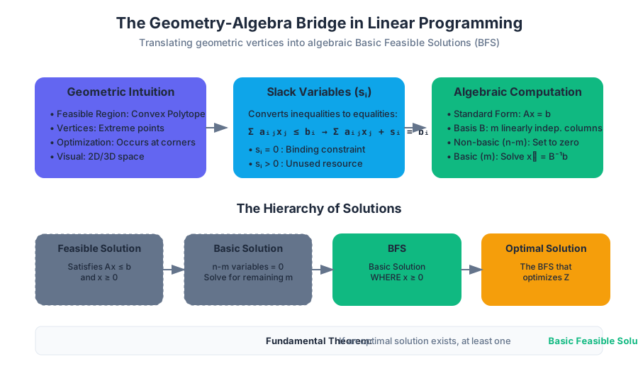
At its core, a Linear Programming Problem (LPP) seeks to optimize a linear objective function subject to linear constraints. Geometrically, the set of all points satisfying these constraints forms a Feasible Region (a convex polytope). The Fundamental Theorem of Linear Programming states that if an optimal solution exists, at least one extreme point (vertex) of the feasible region must be optimal.
To find these vertices algebraically, we use the concept of a BFS. A BFS is essentially the algebraic representation of a vertex.
The Hierarchy of Solutions
| Term | Definition | Geometric Equivalent |
|---|---|---|
| Feasible Solution | Any point $x$ that satisfies all constraints $Ax \le b$ and $x \ge 0$. | Any point inside or on the boundary of the polyhedron. |
| Basic Solution | A solution where $n-m$ variables are set to zero, and the remaining $m$ variables are solved via $Ax = b$. | An intersection point of $n$ constraint hyperplanes. |
| Basic Feasible Solution (BFS) | A Basic Solution that also satisfies the non-negativity constraints ($x \ge 0$). | A vertex (extreme point) of the feasible region. |
| Optimal Solution | A BFS that maximizes or minimizes the objective function. | The "best" vertex. |
Slack Variables: Standardizing the System
Most real-world constraints are inequalities (e.g., "Total labor hours must be less than or equal to 40"). However, linear algebra is built for systems of equations ($Ax = b$). To bridge this gap, we introduce Slack Variables.
Definition and Motivation
A slack variable $s_i$ represents the difference between the left-hand side and the right-hand side of a $\le$ constraint. It quantifies the "unused" portion of a resource.
Definition: Slack Variable For a constraint of the form $\sum a_{ij}x_j \le b_i$, we define a non-negative variable $s_i \ge 0$ such that: $$\sum a_{ij}x_j + s_i = b_i$$ If $s_i = 0$, the constraint is binding (the resource is fully consumed). If $s_i > 0$, the constraint is non-binding.
Transforming to Standard Form
To perform algebraic operations, we must convert the LPP into Standard Form. This requires:
- All constraints are expressed as equalities (using slack or surplus variables).
- All variables are non-negative ($x_i \ge 0$).
- The right-hand side constants are non-negative ($b_i \ge 0$).
Example: Converting to Standard Form
Consider the following non-standard model: Maximize $z = 3x_1 + 2x_2$ Subject to: $2x_1 + x_2 \le 4$ $x_1 + 2x_2 \le 5$ $x_1, x_2 \ge 0$
By adding slack variables $s_1$ and $s_2$, we get the standard form: $2x_1 + x_2 + s_1 = 4$ $x_1 + 2x_2 + s_2 = 5$ $x_1, x_2, s_1, s_2 \ge 0$
Basic and Non-basic Variables
Once in standard form, we have a system of $m$ linear equations with $n$ variables (where $n > m$). This system is underdetermined, meaning it has infinitely many solutions. To find the "corners," we restrict our search.
The $n-m$ Rule
To find a Basic Solution:
- Choose $n-m$ variables and set them to zero. These are called Non-basic Variables (NBV).
- Solve the remaining $m$ equations for the $m$ remaining variables. These are called Basic Variables (BV).
- The set of columns in matrix $A$ corresponding to the basic variables must be Linearly Independent. This set of columns forms a Basis $B$.
Mathematical Representation
Let $A$ be an $m \times n$ matrix of rank $m$. We can partition $A$ into $[B | N]$, where $B$ is an $m \times m$ invertible matrix (the basis) and $N$ is the remaining $m \times (n-m)$ matrix. The equation $Ax = b$ becomes: $$Bx_B + Nx_N = b$$ Setting $x_N = 0$ (Non-basic variables), we solve for $x_B$: $$x_B = B^{-1}b$$
Linear Independence: The Foundation of a Basis
A set of variables can only be "Basic" if their corresponding columns in the constraint matrix $A$ are linearly independent. If the columns are dependent, the matrix $B$ is singular (not invertible), and we cannot solve for a unique $x_B$.
Identifying Linear Independence
As seen in advanced linear algebra (and referenced in Homework 1, Section 0.6), a set of vectors $S = {v_1, v_2, \dots, v_k}$ is linearly independent if the only solution to $c_1v_1 + c_2v_2 + \dots + c_kv_k = 0$ is $c_1 = c_2 = \dots = c_k = 0$.
In the context of BFS, if we pick $m$ columns that are linearly dependent, those variables cannot form a basis. This usually happens when constraints are redundant.
Comparison of Variable States
| State | Variable Type | Value | Interpretation |
|---|---|---|---|
| Non-basic | $x_N$ | Always $0$ | The variable is "at its bound." |
| Basic (Feasible) | $x_B$ | $\ge 0$ | The variable is part of the current solution. |
| Basic (Infeasible) | $x_B$ | $< 0$ | Algebraically valid, but physically impossible (violates $x \ge 0$). |
Implementation: Finding All BFS
While the Simplex method intelligently moves between BFS, a brute-force approach to understanding the concept involves calculating all possible basic solutions and filtering for feasibility.
Python Implementation (NumPy)
This script demonstrates how to extract a basis and solve for basic variables using matrix inversion.
import numpy as np
from itertools import combinations

def find_all_bfs(A, b):
    """
    Finds all Basic Feasible Solutions for a system Ax = b, x >= 0.
    A: m x n matrix
    b: m x 1 vector
    """
    m, n = A.shape
    bfs_list = []

    # Iterate through all possible combinations of m columns
    for indices in combinations(range(n), m):
        B = A[:, indices]

        # Check if the columns are linearly independent (Basis is invertible)
        if np.linalg.matrix_rank(B) == m:
            # Solve B * x_B = b -> x_B = B^-1 * b
            x_b = np.linalg.solve(B, b)

            # Check for feasibility (all components >= 0)
            if np.all(x_b >= -1e-9):  # Using a small epsilon for float precision
                full_solution = np.zeros(n)
                for i, val in enumerate(indices):
                    full_solution[val] = x_b[i]
                bfs_list.append(full_solution)

    return np.unique(bfs_list, axis=0)

# Example: 2x1 + x2 + s1 = 4; x1 + 2x2 + s2 = 5
A_mat = np.array([[2, 1, 1, 0],
                  [1, 2, 0, 1]])
b_vec = np.array([4, 5])

solutions = find_all_bfs(A_mat, b_vec)
print("Basic Feasible Solutions:")
for sol in solutions:
    print(sol)
Mathematical Derivation (LaTeX)
The following block outlines the formal derivation of a Basic Solution.
\text{Given } Ax = b, \text{ partition } x \text{ into } (x_B, x_N):
\begin{pmatrix} B & N \end{pmatrix} \begin{pmatrix} x_B \\ x_N \end{pmatrix} = b

\text{Expand the matrix multiplication:}
B x_B + N x_N = b

\text{Set non-basic variables to zero: } x_N = \mathbf{0}
B x_B + N(\mathbf{0}) = b
B x_B = b

\text{If } B \text{ is non-singular (linearly independent columns):}
x_B = B^{-1}b

\text{The full basic solution is: } x = \begin{pmatrix} B^{-1}b \\ 0 \end{pmatrix}
\text{The solution is Feasible if: } B^{-1}b \ge 0
Worked Example: The "Corner" Hunt
Let's solve for the BFS of the following system:
- $x_1 + x_2 + s_1 = 4$
- $2x_1 + x_2 + s_2 = 6$ $x_1, x_2, s_1, s_2 \ge 0$
Here, $n=4$ (variables) and $m=2$ (constraints). We must set $n-m = 2$ variables to zero.
Case 1: Set $x_1, x_2 = 0$ (Non-basic)
- Basic variables: $s_1, s_2$
- Equations: $s_1 = 4, s_2 = 6$
- Solution: $(0, 0, 4, 6)$. All $\ge 0$, so this is a BFS. (Geometric origin).
Case 2: Set $s_1, s_2 = 0$ (Non-basic)
- Basic variables: $x_1, x_2$
- Equations:
- $x_1 + x_2 = 4$
- $2x_1 + x_2 = 6$
- Subtracting (1) from (2): $x_1 = 2$. Substituting back: $x_2 = 2$.
- Solution: $(2, 2, 0, 0)$. All $\ge 0$, so this is a BFS.
Case 3: Set $x_1, s_1 = 0$ (Non-basic)
- Basic variables: $x_2, s_2$
- Equations:
- $x_2 = 4$
- $x_2 + s_2 = 6 \implies 4 + s_2 = 6 \implies s_2 = 2$
- Solution: $(0, 4, 0, 2)$. All $\ge 0$, so this is a BFS.
Summary of Solutions for this Example
| Combination (NBV) | Basic Variables | Solution $(x_1, x_2, s_1, s_2)$ | Feasible? |
|---|---|---|---|
| ${x_1, x_2}$ | ${s_1, s_2}$ | $(0, 0, 4, 6)$ | Yes |
| ${s_1, s_2}$ | ${x_1, x_2}$ | $(2, 2, 0, 0)$ | Yes |
| ${x_1, s_1}$ | ${x_2, s_2}$ | $(0, 4, 0, 2)$ | Yes |
| ${x_2, s_2}$ | ${x_1, s_1}$ | $(3, 0, 1, 0)$ | Yes |
| ${x_2, s_1}$ | ${x_1, s_2}$ | $(4, 0, 0, -2)$ | No (Infeasible) |
Common Pitfalls and Mastery Checks
When calculating BFS, several technical hurdles can lead to errors. Referring to the Mastery Rubric, a "Mastery+" level understanding requires recognizing these edge cases.
1. Degeneracy
A BFS is degenerate if one or more basic variables equal zero. Geometrically, this means more than $n$ hyperplanes intersect at a single point. This can cause the Simplex method to "cycle" (loop infinitely) unless specific anti-cycling rules (like Bland's Rule) are applied.
2. Linear Dependence
Choosing $m$ columns that are not linearly independent. Error: Attempting to invert a singular matrix. Solution: Ensure the chosen basis $B$ has a non-zero determinant.
3. Infeasibility
Finding a basic solution where $x_i < 0$. Error: Thinking every intersection of lines is a BFS. Reality: Only intersections within the first quadrant (or orthant) are feasible.
4. Standard Form Errors
Forgetting to transform $\ge$ constraints correctly. Correction: For $Ax \ge b$, we subtract a Surplus Variable and add an Artificial Variable to find an initial BFS.
Real-World Usage: Production Libraries
In production environments, we rarely calculate BFS manually. We use highly optimized solvers like Gurobi, CPLEX, or SciPy's linprog. These libraries use the Revised Simplex Method, which maintains the basis $B$ and its inverse efficiently.
Using SciPy for BFS-based Optimization
from scipy.optimize import linprog

# Objective: Maximize 3x1 + 2x2 -> Minimize -3x1 - 2x2
c = [-3, -2]
A = [[2, 1], [1, 2]]
b = [4, 5]
x0_bounds = (0, None)
x1_bounds = (0, None)

res = linprog(c, A_ub=A, b_ub=b, bounds=[x0_bounds, x1_bounds], method='simplex')

print(f"Optimal Value: {-res.fun}")
print(f"Optimal BFS (x1, x2): {res.x}")
# The slack variables can be found in res.slack
print(f"Slack Variables (s1, s2): {res.slack}")
Self-Reflection: Evaluating Your Understanding
Based on the provided grading rubric, assess your work on BFS problems using the following criteria:
| Mastery Level | Criteria |
|---|---|
| Mastery+ | Correctly identifies all BFS, explains degeneracy if present, and provides clear algebraic derivations for $B^{-1}b$. |
| Mastery | Correctly identifies BFS but may have minor transcription errors in the final vector. |
| Developing | Can convert to standard form and add slack variables but struggles with solving the resulting systems or identifying linear independence. |
| Minimal | Understands that slack variables are needed but cannot solve for basic variables algebraically. |
Source Materials
Study Spring 2026 - Math 354 - Sections 02/04 on Lykke
This course page is free to open: signed out, you can read its first two sections, and signing in, on any plan, opens the rest. The free Lykke Chrome extension syncs your own Canvas courses, so ChatGPT, Claude and Muse can answer from your classes and deadlines. It only reads Canvas.
Add the free extensionSign in to open every sectionAll sections of Spring 2026 - Math 354 - Sections 02/04 · Browse more course pages