From the free course Spring 2026 - Math 354 - Sections 02/04 on Lykke
Applied Optimization: The Diet Problem
Key concepts: Cost Minimization · Nutritional Constraints · Standard Form Conversion · Real-world Modeling
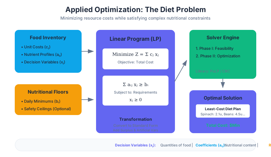
A classic application of linear programming to minimize costs while meeting nutritional requirements.
Applied Optimization: The Diet Problem
The Diet Problem is a foundational archetype in the field of Linear Programming (LP) and operations research. Originally formulated in the 1930s and famously analyzed by Nobel laureate George Stigler in 1945, the problem seeks to identify the most cost-effective combination of foods that satisfies a specific set of nutritional requirements. While it may appear trivial in a modern context of abundance, the Diet Problem represents the birth of systematic resource allocation and remains the template for industrial blending, logistics, and supply chain optimization.
1. The Mathematical Foundation
At its core, the Diet Problem is a constrained optimization problem. We aim to minimize a linear cost function subject to a system of linear inequalities representing nutritional floors (and sometimes ceilings).
1.1 Formal Definition
Let $n$ be the number of available food items and $m$ be the number of essential nutrients.
- Let $x_j$ be the quantity of food $j$ to be consumed (the decision variables).
- Let $c_j$ be the cost per unit of food $j$.
- Let $a_{ij}$ be the amount of nutrient $i$ contained in one unit of food $j$.
- Let $b_i$ be the minimum daily requirement of nutrient $i$.
The objective is to:
Minimize $Z = \sum_{j=1}^{n} c_j x_j$
Subject to: $\sum_{j=1}^{n} a_{ij} x_j \ge b_i$ for all $i = 1, \dots, m$ $x_j \ge 0$ for all $j = 1, \dots, n$
1.2 Why It Matters
Beyond human nutrition, this model is used in:
- Animal Feed Formulation: Creating "Least Cost Rations" for livestock.
- Chemical Blending: Mixing raw ores or chemicals to meet a specific grade at minimum cost.
- Portfolio Optimization: Selecting assets to meet a target return while minimizing risk or cost.
- Energy Grids: Balancing power sources to meet demand at the lowest price point.
2. Standard vs. Canonical Form Conversion
In computational optimization, solvers often require problems to be in a specific format. Most textbook algorithms (like the Simplex method) assume a Standard Form or Canonical Form. Understanding the distinction is critical for debugging solver errors.
| Feature | Standard Form | Canonical Form |
|---|---|---|
| Objective | Usually Maximization | Can be Min or Max |
| Constraints | All equalities ($=$) | All inequalities ($\le$ or $\ge$) |
| Variables | All non-negative ($x_i \ge 0$) | All non-negative ($x_i \ge 0$) |
| Right-Hand Side | Non-negative ($b_i \ge 0$) | No restriction |
2.1 Transformation Mechanics
To convert a Diet Problem (typically a minimization with $\ge$ constraints) into Standard Form for a Simplex solver, we apply three primary transformations:
- Minimization to Maximization: Multiply the objective function by $-1$. $\min Z \iff \max -Z$.
- Inequality to Equality: Introduce Surplus Variables ($s_i$) and Artificial Variables ($a_i$).
- For a $\ge$ constraint: $a_{i1}x_1 + \dots \ge b_i$ becomes $a_{i1}x_1 + \dots - s_i + a_i = b_i$.
- Handling Unrestricted Variables: If a variable $x$ can be negative, replace it with $x = x^+ - x^-$, where $x^+, x^- \ge 0$.
3. Implementation: Solving with PuLP
For modern applications, we use high-level modeling libraries. Below is a Python implementation using the PuLP library, which abstracts the underlying Simplex or Interior Point solvers.
import pulp

def solve_diet_problem(food_data, nutrient_requirements):
    """
    Solves the Diet Problem using the PuLP library.
    food_data: Dict of food names to their cost and nutrient profile.
    nutrient_requirements: Dict of nutrient names to their minimum levels.
    """
    # 1. Initialize the Problem
    prob = pulp.LpProblem("The_Diet_Problem", pulp.LpMinimize)

    # 2. Define Decision Variables (x_j >= 0)
    food_items = list(food_data.keys())
    food_vars = pulp.LpVariable.dicts("Food", food_items, lowBound=0, cat='Continuous')

    # 3. Define Objective Function: Minimize Total Cost
    prob += pulp.lpSum([food_data[f]['cost'] * food_vars[f] for f in food_items]), "Total_Cost"

    # 4. Define Constraints: Meet Nutritional Minimums
    nutrients = list(nutrient_requirements.keys())
    for n in nutrients:
        prob += (
            pulp.lpSum([food_data[f][n] * food_vars[f] for f in food_items]) >=
            nutrient_requirements[n],
            f"Requirement_{n}"
        )

    # 5. Solve
    status = prob.solve(pulp.PULP_CBC_CMD(msg=0))

    # 6. Extract Results
    if pulp.LpStatus[status] == 'Optimal':
        result = {v.name: v.varValue for v in prob.variables() if v.varValue > 0}
        return result, pulp.value(prob.objective)
    else:
        return None, None

# Example Usage
foods = {
    "Spinach": {"cost": 0.12, "calories": 23, "protein": 2.9},
    "Steak": {"cost": 2.50, "calories": 250, "protein": 26.0},
    "Beans": {"cost": 0.50, "calories": 130, "protein": 8.0}
}
reqs = {"calories": 2000, "protein": 50}

plan, cost = solve_diet_problem(foods, reqs)
print(f"Optimal Plan: {plan}, Total Cost: ${cost:.2f}")
4. Algorithmic Deep-Dive: The Two-Phase Simplex
Because the Diet Problem involves $\ge$ constraints, a basic Simplex method cannot start at the origin ($0,0$) because the origin violates the "minimum requirements" constraints. We must use the Two-Phase Simplex Method.
Phase I: Finding a Feasible Basis
We introduce Artificial Variables ($a_i$) to create an initial identity matrix in the tableau. We then minimize the sum of these artificial variables.
- If the minimum sum is $0$, we have found a feasible starting point for the original problem.
- If the minimum sum is $> 0$, the problem is infeasible (no combination of foods satisfies the requirements).
Phase II: Optimizing the Objective
Once a feasible corner point is found, we drop the artificial variables and proceed with the standard Simplex algorithm to find the cost-minimizing vertex.
\begin{array}{l}
\text{Initial Tableau Construction (Phase I):} \\
\begin{bmatrix}
A & -I_{surplus} & I_{artificial} & | & b \\
0 & 0 & 1 \dots 1 & | & W
\end{bmatrix} \\
\text{Where } W \text{ is the sum of artificial variables to be minimized.}
\end{array}
5. Real-World Modeling Challenges
While the mathematical model is elegant, applying it to real-world human diets reveals several "Gotchas" that senior engineers must account for.
5.1 The "Spinach Trap" (Palatability)
A raw LP model might suggest eating 40 pounds of spinach and nothing else because it is the cheapest way to get Vitamin A and Fiber. To solve this, we add Upper Bound Constraints: $x_{spinach} \le 2.0$ (limit consumption to 2 units per day).
5.2 Integer Constraints
You cannot buy $0.342$ of an egg in a grocery store. This transforms the problem into a Mixed-Integer Linear Program (MILP), which is significantly harder to solve (NP-hard) than a standard LP.
5.3 Data Retrieval
In production environments, nutritional data is rarely hardcoded. It is pulled from relational databases.
-- Fetching nutritional data for the optimization engine
SELECT
    f.food_name,
    f.unit_cost,
    n.calories_per_unit,
    n.protein_per_unit,
    n.fat_per_unit
FROM inventory AS f
JOIN nutrition_profiles AS n ON f.food_id = n.food_id
WHERE f.in_stock = 1 AND f.unit_cost IS NOT NULL;
6. Worked Example: The "Mini-Diet"
Let's solve a manual iteration for a simplified case.
Data:
| Food | Cost ($) | Energy (kcal) | Protein (g) |
|---|---|---|---|
| Oatmeal | 0.30 | 150 | 5 |
| Milk | 0.40 | 100 | 8 |
| Target | Min Cost | $\ge$ 300 kcal | $\ge$ 20 g |
Step 1: Formulate Minimize $Z = 0.3x_1 + 0.4x_2$ Subject to:
- $150x_1 + 100x_2 \ge 300$ (Energy)
- $5x_1 + 8x_2 \ge 20$ (Protein)
- $x_1, x_2 \ge 0$
Step 2: Identify Vertices The feasible region is bounded by the intersection of these lines.
- Intersection of (1) and (2):
- $150x_1 + 100x_2 = 300 \implies 3x_1 + 2x_2 = 6$
- $5x_1 + 8x_2 = 20$
- Solving the system: $x_1 \approx 0.57, x_2 \approx 2.14$. Cost: $0.3(0.57) + 0.4(2.14) = \text{\textdollar}1.027$
- Intercepts:
- $x_1$ intercept (where $x_2=0$): $\max(300/150, 20/5) = 4$. Cost: $0.3(4) = \text{\textdollar}1.20$
- $x_2$ intercept (where $x_1=0$): $\max(300/100, 20/8) = 3$. Cost: $0.4(3) = \text{\textdollar}1.20$
Conclusion: The optimal solution is to mix approximately 0.57 units of Oatmeal and 2.14 units of Milk.
7. Common Pitfalls and Error Classification
Based on standard mastery rubrics, errors in the Diet Problem usually fall into three categories:
| Error Type | Description | Example |
|---|---|---|
| Modeling Error | Incorrectly translating units or directions. | Setting a protein constraint as $\le$ instead of $\ge$. |
| Transformation Error | Failing to correctly convert to Standard Form. | Forgetting to subtract the surplus variable in a $\ge$ constraint. |
| Infeasibility Blindness | Failing to recognize when constraints are contradictory. | Requiring 3000 calories but setting a "Max Weight" constraint that allows only 1lb of celery. |
7.1 Debugging Infeasibility
If your solver returns "Infeasible," use the following checklist:
- Check Units: Are you comparing milligrams of Sodium to grams of Protein?
- Relax Constraints: Temporarily remove constraints one by one to find the "bottleneck" nutrient.
- Variable Bounds: Ensure $x_j \ge 0$ is explicitly stated; otherwise, the solver might "eat" negative food to generate nutrients.
8. Extensions: Duality and Shadow Prices
One of the most powerful aspects of the Diet Problem is its Dual.
- Primal: Find the cheapest food mix.
- Dual: Find the "value" (shadow price) of each nutrient.
The Shadow Price of a nutrient tells you how much the total cost would change if the requirement for that nutrient increased by one unit. If the shadow price of Vitamin C is high, it suggests that Vitamin C is the primary driver of your diet's cost. This is invaluable for industrial procurement—it tells the buyer exactly which nutrient-rich ingredients are worth a premium.
# Example: Running a sensitivity analysis via a CLI wrapper
$ diet-solver --input data.json --analyze-shadow-prices

Nutrient       | Shadow Price | Sensitivity Range
-------------------------------------------------
Protein        | 0.05         | [45g, 62g]
Calories       | 0.0002       | [1800, 2500]
Vitamin A      | 1.20         | [0, 5000IU]

# Insight: Vitamin A is the "bottleneck". Reducing its requirement
# by 1 unit saves $1.20.
Summary of Mastery
To achieve Mastery+ in Applied Optimization:
- Formulate the problem with clear decision variables and units.
- Convert the model between Standard, Canonical, and Slack forms without sign errors.
- Implement the solution using professional-grade libraries (PuLP, SciPy, or Gurobi).
- Interpret the results, including shadow prices and feasibility ranges, to provide actionable business or biological insights.
Source Materials
Study Spring 2026 - Math 354 - Sections 02/04 on Lykke
This course page is free to open: signed out, you can read its first two sections, and signing in, on any plan, opens the rest. The free Lykke Chrome extension syncs your own Canvas courses, so ChatGPT, Claude and Muse can answer from your classes and deadlines. It only reads Canvas.
Add the free extensionSign in to open every sectionAll sections of Spring 2026 - Math 354 - Sections 02/04 · Browse more course pages