From the free course Precalculus 2e on Lykke
Polynomial and Rational Functions
Key concepts: Quadratic Functions · Zeros of Polynomials · Rational Functions · Asymptotes
Exploration of higher-degree functions, including quadratics, power functions, and the behavior of rational expressions and their asymptotes.
Polynomial and Rational Functions
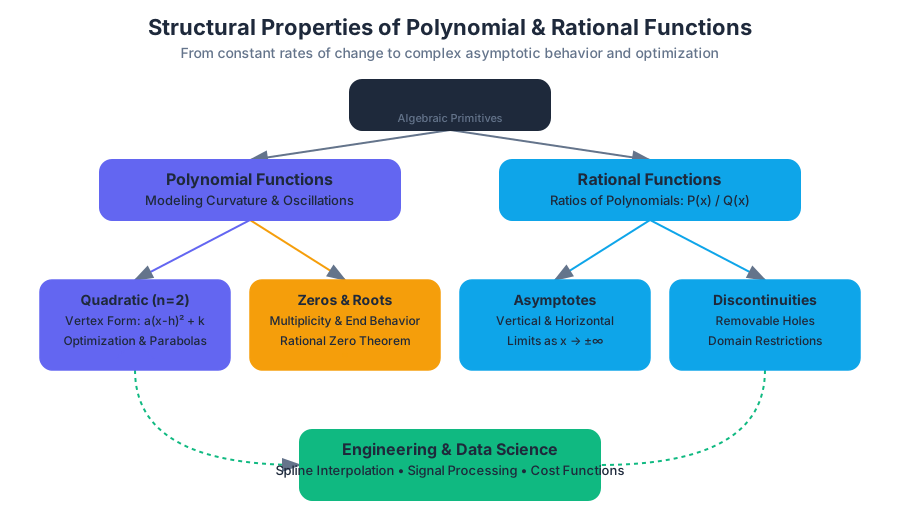
The transition from linear modeling to polynomial and rational functions marks a critical juncture in mathematical maturity. While linear functions describe constant rates of change, Polynomial Functions allow for the modeling of acceleration, curvature, and complex oscillations. Rational Functions, defined as the ratio of two polynomials, introduce the concept of asymptotic behavior and discontinuities—concepts that form the bedrock of calculus and complex analysis.
In the context of modern engineering and data science, these functions are not merely abstract constructs; they are the primitives used in spline interpolation, signal processing, and the optimization of cost functions.
Quadratic Functions and Optimization
A Quadratic Function is a polynomial function of degree 2. Its graph is a parabola, a symmetrical curve that represents the simplest non-linear relationship where the rate of change is itself changing at a constant rate.
1. Definitions and Forms
The utility of a quadratic function often depends on the algebraic form in which it is expressed.
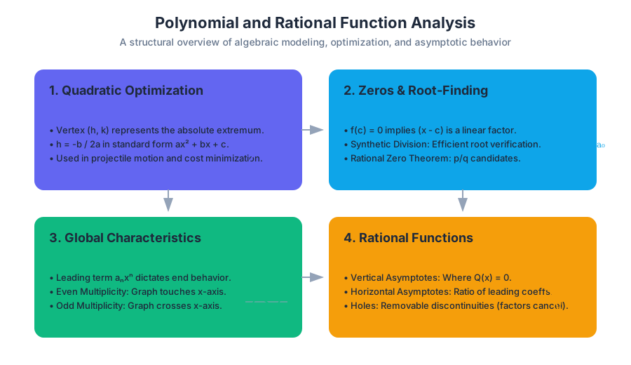
The Vertex Form: $f(x) = a(x - h)^2 + k$ This form is computationally superior for identifying the Vertex $(h, k)$, which represents the absolute maximum or minimum of the function. The value of $a$ determines the "stretch" and the direction of the opening (upward if $a > 0$, downward if $a > 0$).
2. Mechanics of the Vertex
The vertex is the critical point where the function's derivative is zero. In the standard form $f(x) = ax^2 + bx + c$, the x-coordinate of the vertex is derived via $h = -b / (2a)$. Substituting $h$ back into the function yields the y-coordinate $k$.
| Feature | General Form: $ax^2 + bx + c$ | Vertex Form: $a(x-h)^2 + k$ |
|---|---|---|
| Y-Intercept | $(0, c)$ | Found by calculating $f(0)$ |
| Vertex | $(-b/2a, f(-b/2a))$ | $(h, k)$ |
| Axis of Symmetry | $x = -b/2a$ | $x = h$ |
| Optimization | Requires calculation | Immediately visible |
Zeros of Polynomial Functions
As we move to higher-degree polynomials ($n > 2$), the complexity of finding zeros (or roots) increases. A zero of a function $f$ is a value $c$ such that $f(c) = 0$.
1. The Remainder and Factor Theorems
These theorems bridge the gap between polynomial division and function evaluation.
- Remainder Theorem: If a polynomial $f(x)$ is divided by $(x - c)$, the remainder is the value $f(c)$.
- Factor Theorem: A polynomial $f(x)$ has a factor $(x - c)$ if and only if $f(c) = 0$.
2. The Rational Zero Theorem
For a polynomial with integer coefficients, any rational zero must be of the form $p/q$, where $p$ is a factor of the constant term and $q$ is a factor of the leading coefficient. This significantly narrows the search space for roots in high-degree equations.
3. Synthetic Division: The Algorithm
Synthetic division is a shorthand method of polynomial division, specifically for the case of dividing by a linear factor $(x - c)$. It is computationally efficient and forms the basis for many root-finding algorithms.
ALGORITHM: Synthetic Division of P(x) by (x - c)
-----------------------------------------------
Input: Coefficients of P(x) = [a_n, a_{n-1}, ..., a_0], constant c
Output: Quotient coefficients [q_{n-1}, ..., q_0], Remainder r

1. Let current_val = a_n
2. Store a_n as the first coefficient of the quotient.
3. For i from n-1 down to 0:
    a. Multiply current_val by c.
    b. Add result to a_i.
    c. current_val = result + a_i
    d. If i > 0, store current_val as next quotient coefficient.
    e. If i == 0, current_val is the Remainder.
4. End Behavior and Multiplicity
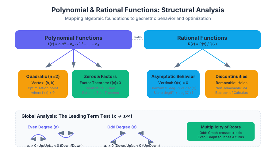
The global shape of a polynomial is dictated by its Leading Term $a_n x^n$. As $x \to \pm \infty$, the leading term dominates all other terms.
| Degree ($n$) | Leading Coeff ($a_n$) | Left Behavior ($x \to -\infty$) | Right Behavior ($x \to \infty$) |
|---|---|---|---|
| Even | Positive (+) | $f(x) \to \infty$ | $f(x) \to \infty$ |
| Even | Negative (-) | $f(x) \to -\infty$ | $f(x) \to -\infty$ |
| Odd | Positive (+) | $f(x) \to -\infty$ | $f(x) \to \infty$ |
| Odd | Negative (-) | $f(x) \to \infty$ | $f(x) \to -\infty$ |
Multiplicity refers to how many times a specific factor $(x - c)$ is repeated. If the multiplicity is even, the graph "touches" the x-axis and turns around. If odd, the graph crosses the x-axis.
Rational Functions and Asymptotic Analysis
A Rational Function is defined as $f(x) = \frac{P(x)}{Q(x)}$, where $P$ and $Q$ are polynomials. These functions introduce "breaks" in the graph where the denominator $Q(x) = 0$.
1. Vertical Asymptotes and Holes
A rational function is undefined when $Q(x) = 0$. However, the nature of this undefined point depends on whether the factor also exists in the numerator.
- Vertical Asymptote: Occurs at $x = c$ if $Q(c) = 0$ and the factor $(x - c)$ does not cancel out with a factor in $P(x)$. The function approaches $\pm \infty$ as it nears $c$.
- Removable Discontinuity (Hole): Occurs at $x = c$ if the factor $(x - c)$ cancels out between $P(x)$ and $Q(x)$. The graph looks continuous except for a single missing point.
2. Horizontal and Slant Asymptotes
Horizontal asymptotes describe the End Behavior of the rational function. They are determined by comparing the degree of the numerator ($n$) to the degree of the denominator ($m$).
| Condition | Asymptote Location | Description |
|---|---|---|
| $n < m$ | $y = 0$ | The x-axis is the horizontal asymptote. |
| $n = m$ | $y = a_n / b_m$ | The ratio of leading coefficients. |
| $n = m + 1$ | Slant (Oblique) | Found using long division; $y = \text{quotient}$. |
| $n > m + 1$ | No Horizontal/Slant | The function behaves like a polynomial of degree $n-m$. |
Inverses and Domain Restriction
An Inverse Function $f^{-1}(x)$ "reverses" the operation of $f(x)$. For an inverse to exist as a function, the original function must be One-to-One (passing the Horizontal Line Test).
1. Restricting the Domain
Most polynomials (like $f(x) = x^2$) are not one-to-one. To find an inverse, we must restrict the domain. For $f(x) = x^2$, we typically restrict $x \geq 0$, allowing the inverse $f^{-1}(x) = \sqrt{x}$ to exist.
2. Algebraic Method for Inverses
- Replace $f(x)$ with $y$.
- Interchange $x$ and $y$.
- Solve for $y$.
- Replace $y$ with $f^{-1}(x)$.
3. Complexity in Rational Inverses
Finding the inverse of a rational function often requires cross-multiplication and factoring to isolate the variable.
Common Pitfalls and Misconceptions
Understanding these functions requires avoiding several "traps" that even advanced students fall into.
| Pitfall | Explanation | Correction |
|---|---|---|
| Canceling Factors | Assuming a canceled factor $(x-c)$ means the function is defined at $c$. | A canceled factor creates a hole, not a point of continuity. |
| Asymptote Crossing | Believing a graph can never cross a horizontal asymptote. | Graphs can cross horizontal asymptotes in the short term; the asymptote only dictates behavior as $x \to \infty$. |
| Leading Term Neglect | Forgetting the sign of the leading coefficient in end behavior. | Always check the sign; a negative $a_n$ flips the entire graph vertically. |
| Complex Roots | Ignoring complex roots because they don't appear on the x-axis. | Complex roots are essential for the Fundamental Theorem of Algebra, which states a degree $n$ polynomial has $n$ roots. |
Summary of the DEI Framework in Precalculus
In alignment with the OpenStax Precalculus 2e philosophy, the study of these functions is presented through a lens of accessibility and diverse representation. By using real-world examples that span various industries—from environmental science (modeling pollutant decay with rational functions) to social science (modeling population growth with polynomials)—the curriculum ensures that the mathematical concepts are grounded in a global context. This approach reduces barriers to entry in STEM by demonstrating the universal utility of algebraic modeling.
Source Materials
Study Precalculus 2e on Lykke
This course page is free to open: signed out, you can read its first two sections, and signing in, on any plan, opens the rest. The free Lykke Chrome extension syncs your own Canvas courses, so ChatGPT, Claude and Muse can answer from your classes and deadlines. It only reads Canvas.
Add the free extensionSign in to open every section