From the free course Precalculus 2e on Lykke
Functions and Linear Modeling
Key concepts: Function Notation · Domain and Range · Rates of Change · Linear Transformations
An introduction to the fundamental building blocks of precalculus, focusing on function notation, domain and range, and the properties of linear functions.
Functions and Linear Modeling
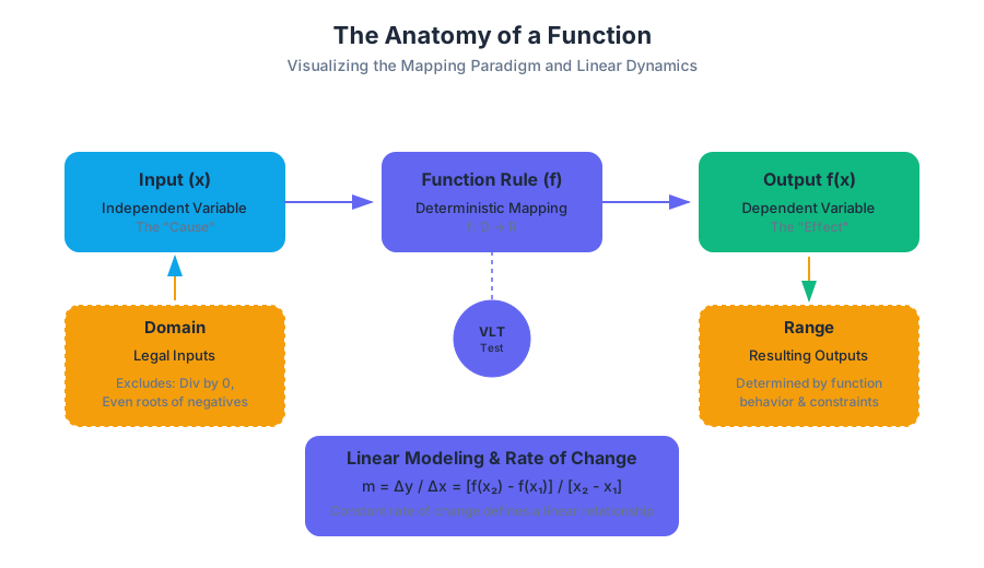
In the hierarchy of mathematical analysis, the function serves as the fundamental unit of mapping. It is the formalization of "relationship"—a deterministic rule that assigns each element from a set of inputs to exactly one element in a set of outputs. While elementary algebra treats equations as static balances to be solved, precalculus shifts the perspective toward functional analysis, where we examine how change in one variable propagates through a system to affect another.
This section explores the mechanics of functions, the constraints of their domains, the dynamics of their rates of change, and the foundational application of Linear Modeling. By mastering these concepts, we move from solving for $x$ to understanding the behavior of $f(x)$.
Function Notation and the Mapping Paradigm
At its core, a function is a specialized type of relation. While all functions are relations, not all relations are functions. The distinguishing characteristic is the uniqueness of the output.
Definition: The Function A function $f$ is a relation that assigns to each element $x$ in a set $D$ (the domain) exactly one element $y$ in a set $R$ (the range). This is notationally represented as $f: D \to R$.
The transition to Function Notation ($f(x)$) is often the first hurdle for students. It is crucial to view $f(x)$ not as "f times x," but as "the value of the output $f$ when the input is $x$." This notation allows for the clear expression of complex operations, such as composition and transformation, which are cumbersome in $y = \dots$ format.
The Vertical Line Test (VLT)
In a Cartesian coordinate system, a relation is a function if and only if no vertical line intersects its graph more than once. This is the visual manifestation of the "one output per input" rule. If a vertical line hits two points, the same $x$ has two different $y$ values, violating the definition of a function.
Evaluating and Simplifying Functions
Evaluating a function involves substituting a specific value or expression into every instance of the independent variable. This often requires algebraic manipulation, particularly when dealing with difference quotients or composite expressions.
| Concept | Notation | Description |
|---|---|---|
| Input | $x$ | The independent variable; the "cause." |
| Output | $f(x)$ | The dependent variable; the "effect." |
| Rule | $f$ | The specific mapping or algorithm applied to $x$. |
| Mapping | $x \mapsto f(x)$ | The process of transforming input to output. |
Domain and Range: The Constraints of Reality
The Domain of a function is the set of all possible "legal" inputs. In pure mathematics, the domain is restricted by the algebraic properties of the real numbers. In applied modeling, the domain is further restricted by the physical or logical constraints of the problem.
Algebraic Restrictions
There are two primary "sins" in real-numbered algebra that define the domain of most functions:
- Division by Zero: Any input that results in a zero denominator must be excluded.
- Even Roots of Negative Numbers: In the real number system, the radicand of an even-indexed root must be non-negative ($\geq 0$).
Interval Notation
To describe these sets efficiently, we use Interval Notation. This system uses brackets [] for inclusive boundaries (where the endpoint is part of the set) and parentheses () for exclusive boundaries.
| Set Description | Inequality | Interval Notation |
|---|---|---|
| Values between $a$ and $b$, inclusive | $a \le x \le b$ | $[a, b]$ |
| Values greater than $a$ | $x > a$ | $(a, \infty)$ |
| All real numbers except $c$ | $x \neq c$ | $(-\infty, c) \cup (c, \infty)$ |
| Values less than or equal to $b$ | $x \le b$ | $(-\infty, b]$ |
The Range is the set of all possible output values. While the domain is often found by looking for what $x$ cannot be, the range is often found by observing the behavior of the function (e.g., the minimum value of a parabola or the horizontal asymptote of a rational function).
Rates of Change: The Dynamics of Functions
A function describes a state, but the Rate of Change describes the motion between states. This concept is the conceptual bridge to the Derivative in Calculus.
Average Rate of Change (AROC)
The average rate of change of a function $f$ over an interval $[x_1, x_2]$ is the ratio of the change in the output values to the change in the input values. Geometrically, this is the slope of the secant line connecting two points on the graph.
$$AROC = \frac{\Delta y}{\Delta x} = \frac{f(x_2) - f(x_1)}{x_2 - x_1}$$
The Difference Quotient
To find the rate of change at a specific point (the instantaneous rate of change), we use the Difference Quotient. This formula calculates the average rate of change between a point $x$ and a point slightly further away, $x+h$.
\text{Difference Quotient} = \frac{f(x + h) - f(x)}{h}, \quad h \neq 0
In Calculus, we take the limit as $h$ approaches zero to find the derivative. In Precalculus, we focus on the algebraic simplification of this expression, which is a critical skill for future success in analysis.
Worked Example: Difference Quotient
For $f(x) = x^2 + 3x$:
- $f(x+h) = (x+h)^2 + 3(x+h) = x^2 + 2xh + h^2 + 3x + 3h$
- $f(x+h) - f(x) = (x^2 + 2xh + h^2 + 3x + 3h) - (x^2 + 3x) = 2xh + h^2 + 3h$
- $\frac{2xh + h^2 + 3h}{h} = 2x + h + 3$
As $h \to 0$, the rate of change becomes $2x + 3$.
Linear Functions and Modeling
A Linear Function is a function with a constant rate of change. This is the simplest form of modeling, where the output changes by a fixed amount for every unit increase in the input.
Forms of Linear Equations
Different contexts require different algebraic representations of lines.
| Form | Equation | Primary Use Case |
|---|---|---|
| Slope-Intercept | $f(x) = mx + b$ | Graphing and identifying the starting value ($b$). |
| Point-Slope | $y - y_1 = m(x - x_1)$ | Constructing a model from a known point and rate. |
| General Form | $Ax + By = C$ | Analyzing intercepts and linear programming. |
Modeling Real-World Data
Linear modeling involves identifying the initial value (the y-intercept) and the constant rate (the slope).
Example: Telecommunications Pricing A data plan costs $30 per month plus $5 per gigabyte of data used. Here, $b = 30$ (fixed cost) and $m = 5$ (variable rate). The model is $C(g) = 5g + 30$.
Linear Regression
When data points do not fall perfectly on a line, we use Linear Regression to find the "Line of Best Fit." This minimizes the sum of the squares of the vertical deviations (residuals) between the data points and the line.
Linear Transformations: Manipulating Function Geometry
Transformations allow us to create a family of functions based on a "parent" function. By applying constants to the input or output, we can shift, scale, or reflect the graph.
Vertical and Horizontal Shifts
- Vertical Shift: $g(x) = f(x) + k$. If $k > 0$, the graph moves up; if $k < 0$, it moves down.
- Horizontal Shift: $g(x) = f(x - h)$. If $h > 0$, the graph moves right; if $h < 0$, it moves left. (Note the subtraction in the formula).
Scaling and Reflections
- Vertical Stretch/Compression: $g(x) = a f(x)$. If $|a| > 1$, it stretches; if $0 < |a| < 1$, it compresses.
- Horizontal Stretch/Compression: $g(x) = f(bx)$. If $|b| > 1$, it compresses horizontally; if $0 < |b| < 1$, it stretches horizontally.
- Reflections: $-f(x)$ reflects across the x-axis; $f(-x)$ reflects across the y-axis.
Summary of Transformations
| Operation | Transformation | Effect on $(x, y)$ |
|---|---|---|
| $f(x) + k$ | Vertical Shift | $(x, y + k)$ |
| $f(x - h)$ | Horizontal Shift | $(x + h, y)$ |
| $a f(x)$ | Vertical Scale | $(x, ay)$ |
| $f(bx)$ | Horizontal Scale | $(x/b, y)$ |
| $-f(x)$ | Reflection (x-axis) | $(x, -y)$ |
| $f(-x)$ | Reflection (y-axis) | $(-x, y)$ |
Common Pitfalls and Edge Cases
- Confusing $f(x+h)$ with $f(x)+h$: The former is a horizontal shift (input modification), while the latter is a vertical shift (output modification).
- Order of Transformations: When multiple transformations are applied, the order matters. Generally, follow the order of operations: perform horizontal shifts, then horizontal scaling, then reflections, then vertical scaling, and finally vertical shifts.
- Domain of Composite Functions: The domain of $f(g(x))$ is not just the domain of the final simplified expression. It must also exclude any values that are not in the domain of the inner function $g(x)$.
- Slope of Vertical Lines: A vertical line has an "undefined" slope because $\Delta x = 0$. Consequently, vertical lines are not functions of $x$.
Source Materials
Study Precalculus 2e on Lykke
This course page is free to open: signed out, you can read its first two sections, and signing in, on any plan, opens the rest. The free Lykke Chrome extension syncs your own Canvas courses, so ChatGPT, Claude and Muse can answer from your classes and deadlines. It only reads Canvas.
Add the free extensionSign in to open every section