From the free course Precalculus 2e on Lykke
Analytic Geometry and Intro to Calculus
Key concepts: Conic Sections · Sequences and Series · Limits · Continuity
Advanced topics including conic sections, sequences, and a foundational introduction to the concept of limits.
Analytic Geometry and Intro to Calculus
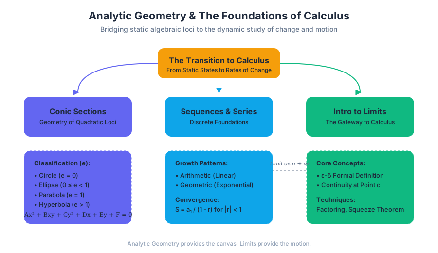
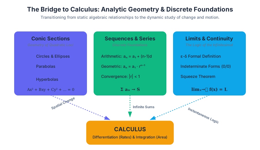
The transition from Precalculus to Calculus represents a fundamental shift in mathematical maturity. While algebra and trigonometry focus on static relationships—solving for $x$ in a fixed state—Calculus introduces the study of change and motion. This section serves as the bridge, formalizing the geometry of curves (Conic Sections), the behavior of discrete patterns (Sequences and Series), and the foundational logic of the infinitesimal (Limits and Continuity).
Conic Sections: The Geometry of Quadratic Loci
Conic sections are the curves obtained by the intersection of a plane with a double-napped right circular cone. Historically, these were studied by Apollonius of Perga, but their modern utility in orbital mechanics, acoustics, and optics stems from their description as algebraic loci.
The General Second-Degree Equation
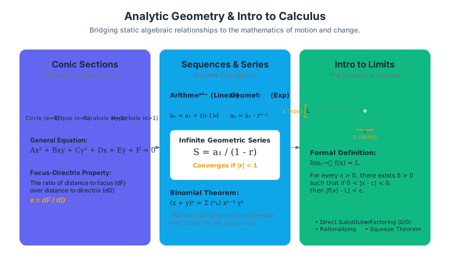
Any conic section can be represented by the general equation: $$Ax^2 + Bxy + Cy^2 + Dx + Ey + F = 0$$ The type of conic is determined by the discriminant $B^2 - 4AC$. In the standard Precalculus curriculum, we often focus on the "non-rotated" case where $B=0$.
| Conic Section | Geometric Definition (Locus) | Standard Equation (Center at $h,k$) | Eccentricity ($e$) |
|---|---|---|---|
| Parabola | Points equidistant from a focus and a directrix. | $(x-h)^2 = 4p(y-k)$ | $e = 1$ |
| Ellipse | Points where the sum of distances to two foci is constant. | $\frac{(x-h)^2}{a^2} + \frac{(y-k)^2}{b^2} = 1$ | $0 \le e < 1$ |
| Hyperbola | Points where the difference of distances to two foci is constant. | $\frac{(x-h)^2}{a^2} - \frac{(y-k)^2}{b^2} = 1$ | $e > 1$ |
| Circle | Points at a constant distance from a center. | $(x-h)^2 + (y-k)^2 = r^2$ | $e = 0$ |
Eccentricity and Directrix
The eccentricity ($e$) of a conic section measures how much the conic deviates from being a circle. It is defined as the ratio of the distance from any point on the conic to the focus ($d_F$) and the distance to the directrix ($d_D$): $e = d_F / d_D$.
The Focus-Directrix Property: For any conic section (except the circle), the ratio of the distance from a point $P$ to a fixed point (focus) to the distance from $P$ to a fixed line (directrix) is a constant $e$.
Sequences and Series: Discrete Foundations
Sequences are ordered lists of numbers, while series represent the sum of those numbers. In the context of Calculus, sequences provide the discrete framework for understanding limits as $n \to \infty$.
Arithmetic vs. Geometric Progressions
- Arithmetic Sequence: Each term is the previous term plus a constant $d$ (common difference).
- $n$-th term: $a_n = a_1 + (n-1)d$
- Sum ($S_n$): $\frac{n}{2}(a_1 + a_n)$
- Geometric Sequence: Each term is the previous term multiplied by a constant $r$ (common ratio).
- $n$-th term: $a_n = a_1 \cdot r^{n-1}$
- Sum ($S_n$): $\frac{a_1(1-r^n)}{1-r}$
Convergence of Infinite Series
An infinite geometric series converges if and only if $|r| < 1$. If it converges, the sum is: $$S = \frac{a_1}{1-r}$$ This concept is the precursor to the Taylor Series in Calculus II, where functions are represented as infinite sums of polynomials.
| Feature | Arithmetic | Geometric |
|---|---|---|
| Recursive Formula | $a_n = a_{n-1} + d$ | $a_n = a_{n-1} \cdot r$ |
| Growth Pattern | Linear | Exponential |
| Infinite Sum | Always Diverges (unless $a_i=0$) | Converges if $|r| < 1$ |
| Common Application | Simple Interest, Depreciation | Compound Interest, Fractals |
\text{The Binomial Theorem expansion for } (x+y)^n:
(x+y)^n = \sum_{k=0}^{n} \binom{n}{k} x^{n-k} y^k
\text{where } \binom{n}{k} = \frac{n!}{k!(n-k)!}
Introduction to Limits: The Gateway to Calculus
The limit is the single most important concept in calculus. It allows us to describe the behavior of a function as the input approaches a value, even if the function is undefined at that specific point.
Formal Definition ($\epsilon-\delta$)
While the intuitive definition is "the value $f(x)$ gets close to," the rigorous definition (the Weierstrass definition) is:
Let $f(x)$ be defined on an open interval containing $c$ (except possibly at $c$). We say $\lim_{x \to c} f(x) = L$ if for every $\epsilon > 0$, there exists a $\delta > 0$ such that if $0 < |x - c| < \delta$, then $|f(x) - L| < \epsilon$.
This definition is essentially a "challenge-response" game: if you tell me how close you want the output to be to $L$ (the $\epsilon$), I can tell you how close $x$ must be to $c$ (the $\delta$).
Limit Laws and Algebraic Manipulation
Evaluating limits often requires bypassing "indeterminate forms" like $0/0$ or $\infty/\infty$.
| Technique | When to Use | Example |
|---|---|---|
| Direct Substitution | For continuous functions. | $\lim_{x \to 2} x^2 = 4$ |
| Factoring | When substitution yields $0/0$. | $\frac{x^2-4}{x-2} \to \frac{(x-2)(x+2)}{x-2}$ |
| Rationalizing | When square roots create $0/0$. | Multiply by the conjugate. |
| Squeeze Theorem | When the function is "trapped" between two others. | $\lim_{x \to 0} x^2 \sin(1/x) = 0$ |
Continuity: The Absence of Breaks
A function is continuous if its graph can be drawn without lifting the pencil. However, in technical terms, continuity at a point requires three distinct conditions to be met.
The Three-Part Definition of Continuity
A function $f(x)$ is continuous at $x = c$ if:
- $f(c)$ is defined (the point exists).
- $\lim_{x \to c} f(x)$ exists (the left-hand and right-hand limits match).
- $\lim_{x \to c} f(x) = f(c)$ (the limit equals the point).
Types of Discontinuity
Understanding where a function fails to be continuous is critical for identifying system instabilities or "shocks" in physical models.
| Type | Description | Graphical Representation |
|---|---|---|
| Removable | A "hole" in the graph; the limit exists but the point doesn't match. | A line with a single missing dot. |
| Jump | The left and right limits exist but are not equal. | Common in piecewise/step functions. |
| Infinite | The function approaches $\pm \infty$ as $x$ approaches $c$. | A vertical asymptote. |
The Intermediate Value Theorem (IVT)
The IVT is a powerful existence theorem:
If $f$ is continuous on a closed interval $[a, b]$, and $k$ is any number between $f(a)$ and $f(b)$, then there exists at least one number $c$ in $(a, b)$ such that $f(c) = k$.
Practical Application: The IVT is the mathematical justification for the Bisection Method used in computer science to find roots of equations. If a continuous function changes sign between $a$ and $b$, there must be a zero in between.
Synthesis: Connecting the Dots
The concepts in this section are not isolated. They represent a progression of complexity:
- Conics define the paths of objects (like a planet's orbit).
- Sequences allow us to sample that path at discrete intervals.
- Limits allow us to shrink those intervals to zero.
- Continuity ensures that the path is a smooth, predictable trajectory rather than a series of disjointed teleports.
In Calculus I, you will use the limit to define the Derivative (the slope of a tangent line to a conic) and the Integral (the area under a curve). Without the rigorous definitions of limits and continuity established here, the entire edifice of modern physics and engineering would lack a logical foundation.
Common Pitfalls and Misconceptions
- Limit vs. Value: A common mistake is assuming $\lim_{x \to c} f(x)$ must equal $f(c)$. The limit describes the neighborhood, while $f(c)$ describes the point. They only agree if the function is continuous.
- Divergence of Harmonic Series: Students often assume that if the terms of a series go to zero ($a_n \to 0$), the series must converge. The Harmonic Series ($\sum 1/n$) is the classic counterexample: the terms get smaller, but the sum grows to infinity.
- Hyperbola Asymptotes: Unlike a parabola, which opens wider and wider, a hyperbola is constrained by linear asymptotes $y = \pm \frac{b}{a}(x-h) + k$. Confusing the two leads to significant errors in trajectory modeling.
- The "0/0" Trap: $0/0$ is not 1, and it is not 0. It is indeterminate, meaning more work (factoring, rationalizing) is required to find the actual limit.
Source Materials
Study Precalculus 2e on Lykke
This course page is free to open: signed out, you can read its first two sections, and signing in, on any plan, opens the rest. The free Lykke Chrome extension syncs your own Canvas courses, so ChatGPT, Claude and Muse can answer from your classes and deadlines. It only reads Canvas.
Add the free extensionSign in to open every section