From the free course pandas documentation on Lykke
Reshaping and Combining Datasets
Key concepts: Pivot · Melt · Concat · Merge · Long vs Wide format
Advanced layout changes and merging multiple data sources into a single analysis-ready table.
Reshaping and Combining Datasets
In the lifecycle of data engineering and analysis, raw data rarely arrives in a format ready for immediate consumption. It is often fragmented across disparate sources—SQL databases, CSV logs, or JSON API responses—and structured in ways that prioritize storage efficiency or capture convenience over analytical utility. Reshaping and combining are the fundamental operations used to transform these "wild" datasets into "tidy" structures suitable for machine learning, statistical modeling, and visualization.
AI_SVGI_SVGt its core, reshaping is about changing the layout of a single table to better represent the relationship between variables and observations. Combining is about the integration of multiple tables into a unified whole, ensuring that relational integrity is maintained across different axes of information. Mastering these operations requires an understanding of both the algebraic properties of relational joins and the memory-management implications of data alignment.
The Taxonomy of Data Shapes: Long vs. Wide
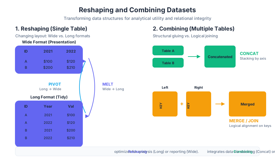
Before applying transformations, one must identify the current and target "shape" of the data. In the context of tabular data, we categorize structures into two primary formats: Long (also known as "stacked" or "tidy") and Wide (also known as "unstacked" or "presentation" format).
Definition: Tidy Data A dataset is considered "tidy" when:
- Each variable forms a column.
- Each observation forms a row.
- Each type of observational unit forms a table.
Comparison of Data Formats
| Feature | Wide Format | Long Format |
|---|---|---|
| Structure | Variables are spread across multiple columns (e.g., Year_2020, Year_2021). |
Variables are stored in a single "Key" column with values in a "Value" column. |
| Readability | High for humans; easy to compare values side-by-side. | Low for humans; repetitive identifiers. |
| Analysis | Difficult for group-by operations or time-series modeling. | Ideal for seaborn plotting, scikit-learn modeling, and SQL-like aggregations. |
| Scalability | Adding a new category requires adding a new column (schema change). | Adding a new category requires adding new rows (no schema change). |
| Memory | Often more compact for sparse data. | Can be memory-intensive due to repeated index/ID labels. |
Reshaping Mechanics: Pivot and Melt
Reshaping is the process of rotating the data's axes. In the Python/Pandas ecosystem, this is primarily handled by pivot, pivot_table, and melt.
Pivot: From Long to Wide
The pivot operation takes unique values from one column and turns them into column headers for a new DataFrame. This is essentially a "de-normalization" step used for reporting or creating correlation matrices.
- Index: The column(s) to use as the new row labels.
- Columns: The column whose unique values will become the new column headers.
- Values: The column(s) whose values will fill the new table cells.
If your data has duplicate entries for the same index/column pair, pivot will fail. In such cases, pivot_table is required, as it allows for an aggregation function (like mean, sum, or count) to resolve collisions.
Melt: From Wide to Long
The melt operation is the inverse of pivot. It "unpivots" a DataFrame from a wide format to a long format, which is often a prerequisite for advanced data cleaning.
- id_vars: Columns that should remain as identifiers (not melted).
- value_vars: Columns to be unpivoted (if not specified, uses all columns not in
id_vars). - var_name: Name for the new "variable" column.
- value_name: Name for the new "value" column.
import pandas as pd
import numpy as np

# Low-level implementation of a Pivot-like transformation using pure Python
# to demonstrate the underlying logic of coordinate mapping.
def manual_pivot(data, index_col, columns_col, values_col):
    """
    Simulates the logic of pd.pivot:
    Maps (row_id, col_id) pairs to a 2D grid.
    """
    # Identify unique coordinates
    unique_indices = sorted(list(set(row[index_col] for row in data)))
    unique_columns = sorted(list(set(row[columns_col] for row in data)))

    # Create mapping for O(1) lookup
    idx_map = {val: i for i, val in enumerate(unique_indices)}
    col_map = {val: i for i, val in enumerate(unique_columns)}

    # Initialize an empty matrix (NaN-filled)
    matrix = np.full((len(unique_indices), len(unique_columns)), np.nan)

    # Fill the matrix
    for entry in data:
        r = idx_map[entry[index_col]]
        c = col_map[entry[columns_col]]
        matrix[r, c] = entry[values_col]

    return matrix, unique_indices, unique_columns

# Example usage with raw dictionary data
raw_data = [
    {'city': 'NYC', 'date': '2023-01-01', 'temp': 32},
    {'city': 'NYC', 'date': '2023-01-02', 'temp': 35},
    {'city': 'LA', 'date': '2023-01-01', 'temp': 70},
    {'city': 'LA', 'date': '2023-01-02', 'temp': 72},
]

pivoted, rows, cols = manual_pivot(raw_data, 'date', 'city', 'temp')
print(f"Columns: {cols}\nRows: {rows}\nMatrix:\n{pivoted}")
AI_DEMOI_DEMO## Combining Datasets: Concatenation and Merging
While reshaping deals with the internal structure of a single dataset, combining deals with the relationship between multiple datasets. We distinguish between Concatenation (structural gluing) and Merging (logical joining).
Concatenation (pd.concat)
Concatenation is the process of "stacking" DataFrames along a particular axis.
- Axis 0 (Rows): Stacking tables vertically. This is common when you have monthly logs (Jan, Feb, Mar) and want a single year-to-date table.
- Axis 1 (Columns): Aligning tables horizontally based on their index.
Concatenation is primarily a structural operation. It does not look at the content of the columns to find matches; it relies on the alignment of labels (indexes or column names).
Merging (pd.merge)
Merging is a relational operation, analogous to SQL JOINs. It combines tables based on the values of one or more "keys."
The Join Theorem Given two sets $L$ (Left) and $R$ (Right), a Join operation $L \bowtie R$ produces a set of tuples $(l, r)$ such that $l \in L, r \in R$ and a predicate $P(l, r)$ is satisfied (usually $l.key = r.key$).
Join Types and Logic
| Join Type | Pandas Argument | SQL Equivalent | Result Description |
|---|---|---|---|
| Inner | how='inner' |
INNER JOIN |
Only keys present in both tables are kept. |
| Left | how='left' |
LEFT OUTER JOIN |
All keys from the left table are kept; right values are NaN if no match. |
| Right | how='right' |
RIGHT OUTER JOIN |
All keys from the right table are kept; left values are NaN if no match. |
| Outer | how='outer' |
FULL OUTER JOIN |
All keys from both tables are kept; missing values are filled with NaN. |
| Cross | how='cross' |
CROSS JOIN |
Cartesian product: every row of left paired with every row of right. |
\begin{aligned}
&\text{Let } A = \{ (k_1, v_1), (k_2, v_2) \} \text{ and } B = \{ (k_1, w_1), (k_3, w_3) \} \\
&\text{Inner Join: } A \cap_k B = \{ (k_1, v_1, w_1) \} \\
&\text{Left Join: } A \cup_k B_{left} = \{ (k_1, v_1, w_1), (k_2, v_2, \text{NaN}) \} \\
&\text{Outer Join: } A \cup_k B = \{ (k_1, v_1, w_1), (k_2, v_2, \text{NaN}), (k_3, \text{NaN}, w_3) \}
\end{aligned}
Merge Implementation in Practice
The power of pd.merge lies in its flexibility regarding key names. If the keys are named differently in each table, we use left_on and right_on.
-- SQL Representation of a complex merge
-- This logic is what pd.merge(df1, df2, left_on='user_id', right_on='id', how='left') executes
SELECT
    df1.user_id,
    df1.purchase_amount,
    df2.user_name,
    df2.signup_date
FROM
    transactions AS df1
LEFT JOIN
    users AS df2
ON
    df1.user_id = df2.id;
Advanced Reshaping: Stack and Unstack
For datasets with Hierarchical Indexing (MultiIndex), Pandas provides the stack() and unstack() methods. These are specialized versions of pivot/melt designed for multi-level labels.
- Stack: "Compresses" a level in the DataFrame's columns to produce a multi-level index (moving from wide to long).
- Unstack: "Expands" a level in the DataFrame's index into the column axis (moving from long to wide).
Comparison: Pivot vs. Stack
| Operation | Best Used When... | Handling of Missing Data |
|---|---|---|
| Pivot | You want to specify exactly which columns become the new index/columns. | Leaves NaN where no match exists. |
| Stack | You have a MultiIndex and want to rotate a specific level. | Automatically drops NaN values by default (dropna=True). |
Common Pitfalls and Performance Considerations
1. The Cartesian Product Explosion
When merging on keys that are not unique in both tables, the resulting DataFrame can grow exponentially. If Table A has 1,000 instances of key=1 and Table B has 1,000 instances of key=1, an inner join will produce 1,000,000 rows for that key alone.
- Fix: Always check for duplicates in your keys using
df.duplicated(subset=['key']).any()before merging.
2. Loss of Integer Dtypes (The NaN Problem)
In Pandas (prior to version 1.0), the standard integer type (int64) did not support NaN. If a merge or pivot introduced missing values, the entire column would be silently cast to float64.
- Fix: Use the nullable integer type
Int64(capital 'I') or ensure data completeness before joining.
3. Memory Fragmentation
Repeatedly concatenating DataFrames in a loop (e.g., for file in files: df = pd.concat([df, pd.read_csv(file)])) is an $O(N^2)$ operation because Pandas creates a new copy of the entire dataset at every iteration.
- Fix: Collect all DataFrames in a list and call
pd.concatonce.
# Performance Tip: Inspecting keys before a merge using CLI tools
# This helps identify if 'user_id' is a viable join key without loading 10GB into RAM.

# Count unique keys in a CSV
cut -d',' -f1 large_data.csv | sort | uniq -c | sort -nr | head -n 10

# Check for null keys in the join column
awk -F',' '$1 == "" {print "Empty key found at line " NR}' large_data.csv
Real-World Workflow: The "Reshape-Combine" Pipeline
Often, a data task requires a sequence of these operations. Consider a scenario where you have weather data in multiple CSVs (one per city) in a wide format, and you need to join it with a central "City Metadata" table.
- Read & Concat: Load all city CSVs and
pd.concatthem into one master wide table. - Melt: Convert the wide table (columns like
Jan,Feb,Mar) into a long table (Month,Temperature). - Merge: Join the long table with the
City_Metadatatable on theCity_IDkey. - Pivot Table: Create a final summary report showing average temperature by
Region(from metadata) andSeason.
AI_STUDY_GUIDEI_STUDY_GUIDE### Summary Table of Operations
| Goal | Primary Method | Key Parameter |
|---|---|---|
| Stack rows vertically | pd.concat([df1, df2]) |
axis=0 |
| Join on shared values | pd.merge(df1, df2) |
on='key_col' |
| Turn rows into columns | df.pivot() |
columns='col_to_rotate' |
| Turn columns into rows | df.melt() |
id_vars=['keep_cols'] |
| Aggregate while pivoting | df.pivot_table() |
aggfunc='mean' |
| Rotate MultiIndex levels | df.stack() / df.unstack() |
level=-1 |
Source Materials
Study pandas documentation on Lykke
This course page is free to open: signed out, you can read its first two sections, and signing in, on any plan, opens the rest. The free Lykke Chrome extension syncs your own Canvas courses, so ChatGPT, Claude and Muse can answer from your classes and deadlines. It only reads Canvas.
Add the free extensionSign in to open every sectionAll sections of pandas documentation · Browse more course pages