From the free course pandas documentation on Lykke
Data Manipulation and Summary Statistics
Key concepts: Vectorization · Split-Apply-Combine · Groupby · Summary Statistics · Renaming
Transforming data through mathematical operations, grouping, and statistical aggregation.
Data Manipulation and Summary Statistics
In the realm of computational data science, the transition from raw, unstructured observations to actionable insights is mediated by two fundamental capabilities: the ability to perform high-performance bulk operations and the ability to reduce high-dimensional data into meaningful summaries. This section explores the mechanics of Vectorization, the conceptual framework of Split-Apply-Combine, and the rigorous application of Summary Statistics within the pandas ecosystem.
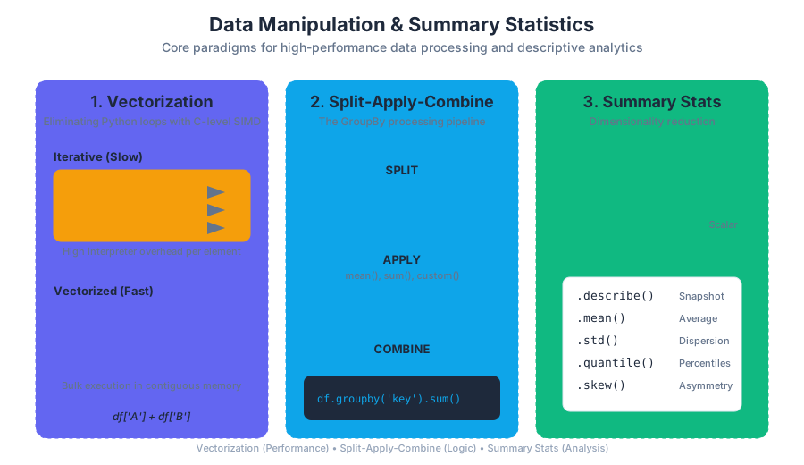
AI_SVGI_SVG## Vectorization: The Engine of Performance
At the heart of pandas lies the principle of Vectorization. In traditional imperative programming, operations on a collection of items are typically handled via explicit loops (e.g., for or while). Vectorization replaces these explicit loops with "array-oriented" operations that occur at the compiled C and Cython levels.
What it is
Vectorization is the process of executing an operation on an entire array (or Series) at once, rather than iterating through individual elements. Mathematically, if we have two vectors $\mathbf{a}$ and $\mathbf{b}$ of length $n$, a vectorized addition $\mathbf{c} = \mathbf{a} + \mathbf{b}$ computes $c_i = a_i + b_i$ for all $i \in {1, \dots, n}$ in a single conceptual step.
Why it matters
Python is an interpreted language, and the overhead of the Python interpreter—type checking, dynamic dispatch, and object creation—within a loop can be orders of magnitude slower than the actual arithmetic operation. Vectorization delegates the loop to highly optimized C or Fortran code (via NumPy), leveraging SIMD (Single Instruction, Multiple Data) instructions at the CPU level.
How it works
When you execute df['A'] + df['B'], pandas does not call the Python + operator $n$ times. Instead, it identifies the underlying memory buffers (NumPy arrays) and passes pointers to these buffers to a pre-compiled C routine. This routine iterates through the contiguous memory blocks, minimizing cache misses and maximizing throughput.
| Feature | Iterative (Loops) | Vectorized (Pandas/NumPy) |
|---|---|---|
| Execution Speed | Slow (High Python overhead) | Fast (C-level execution) |
| Code Readability | Verbose, boilerplate-heavy | Concise, mathematical |
| Memory Access | Frequent pointer chasing | Contiguous memory blocks |
| Type Safety | Checked at every iteration | Checked once per array |
import pandas as pd
import numpy as np
import time

# Generating a dataset with 10 million rows
n = 10_000_000
df = pd.DataFrame({
    'price': np.random.uniform(10, 100, size=n),
    'quantity': np.random.randint(1, 10, size=n)
})

# 1. THE SLOW WAY: Manual Iteration (Anti-pattern)
start = time.time()
total_loop = []
for i in range(len(df)):
    total_loop.append(df.iloc[i]['price'] * df.iloc[i]['quantity'])
end = time.time()
print(f"Loop time: {end - start:.4f} seconds")

# 2. THE FAST WAY: Vectorization
start = time.time()
df['total'] = df['price'] * df['quantity']
end = time.time()
print(f"Vectorized time: {end - start:.4f} seconds")
AI_DEMOI_DEMO## Summary Statistics: Descriptive Analytics
Summary statistics are the primary tools used to describe the distribution, central tendency, and dispersion of a dataset. In pandas, these are implemented as reducing methods that collapse a dimension of a DataFrame or Series into a single scalar value.
The describe() Method
The most comprehensive entry point for summary statistics is the .describe() method. It provides a diagnostic "snapshot" of the data. For numerical data, it returns:
- Count: Number of non-null observations.
- Mean: The arithmetic average.
- Std: Standard deviation (a measure of spread).
- Min/Max: The range boundaries.
- Percentiles: The 25th, 50th (median), and 75th percentiles.
Mathematical Foundations
Pandas uses the "N-1" convention for sample standard deviation by default (Bessel's correction), which provides an unbiased estimate of the population variance from a sample.
s = \sqrt{\frac{\sum_{i=1}^{n} (x_i - \bar{x})^2}{n - 1}}
Where:
- $x_i$ is an individual observation.
- $\bar{x}$ is the sample mean.
- $n$ is the number of observations.
Common Statistical Methods
| Method | Description | SQL Equivalent |
|---|---|---|
.mean() |
Arithmetic mean of values | AVG() |
.median() |
Median (50th percentile) | PERCENTILE_CONT(0.5) |
.std() |
Sample standard deviation | STDEV() |
.var() |
Unbiased variance | VAR() |
.skew() |
Sample skewness (3rd moment) | N/A (Standard) |
.kurt() |
Sample kurtosis (4th moment) | N/A (Standard) |
.quantile(q) |
Value at quantile $q$ | PERCENTILE_DISC(q) |
The Split-Apply-Combine Paradigm
The most powerful pattern in data manipulation is Split-Apply-Combine, a term coined by Hadley Wickham. It describes a strategy where a large problem is broken down into manageable pieces, operated upon, and then reassembled.
Definition: Split-Apply-Combine is a data processing strategy where a dataset is partitioned into groups (Split), a function is executed on each group independently (Apply), and the results are concatenated into a new data structure (Combine).
1. Split
The groupby() function is the primary mechanism for splitting. It creates a GroupBy object, which is a "lazy" representation of the data. No computation happens during the split phase; pandas simply maps the index labels to group identifiers.
2. Apply
Once the data is split, you apply a function. There are three main categories of application:
- Aggregation: Reduces each group to a single value (e.g.,
sum,mean,count). - Transformation: Performs a group-specific computation but returns an object with the same shape as the original (e.g., standardizing data within a group).
- Filtration: Discards entire groups based on a boolean condition (e.g., removing groups with fewer than 100 observations).
3. Combine
Pandas automatically handles the reassembly of the results. If the apply step returns a scalar per group, the result is a Series (or DataFrame if multiple columns were aggregated) with the group keys as the index.
/*
A conceptual representation of Split-Apply-Combine in SQL
This shows how the 'Split' (GROUP BY) and 'Apply' (SUM)
work together to 'Combine' into a result set.
*/

SELECT
    department_id,
    SUM(salary) AS total_payroll,
    AVG(salary) AS avg_salary
FROM
    employees
WHERE
    hire_date > '2020-01-01'
GROUP BY
    department_id
HAVING
    COUNT(*) > 5;
Groupby Mechanics and Syntax
The syntax for groupby in pandas is highly flexible, allowing for grouping by column names, levels of a MultiIndex, or even external arrays.
Aggregation via .agg()
While you can call .sum() directly on a GroupBy object, the .agg() (or .aggregate()) method allows for much more granular control, such as applying different functions to different columns.
Transformation via .transform()
Transformation is often misunderstood. Unlike aggregation, which reduces the number of rows, transformation preserves the original index. This is critical for operations like "percent of group total" or "group-wise imputation."
# Real-world usage: Financial Data Normalization
import pandas as pd

data = {
    'Sector': ['Tech', 'Tech', 'Energy', 'Energy', 'Tech', 'Retail'],
    'Ticker': ['AAPL', 'MSFT', 'XOM', 'CVX', 'NVDA', 'WMT'],
    'Price': [150, 250, 80, 120, 400, 140],
    'MarketCap': [2.5, 2.2, 0.4, 0.3, 1.1, 0.5] # In Trillions
}
df = pd.DataFrame(data)

# 1. Aggregation: What is the total market cap per sector?
sector_totals = df.groupby('Sector')['MarketCap'].sum()

# 2. Transformation: Z-Score of price within each sector
# Formula: (x - mean) / std
z_score = lambda x: (x - x.mean()) / x.std()
df['Sector_Z_Score'] = df.groupby('Sector')['Price'].transform(z_score)

# 3. Filtration: Keep only sectors with more than 1 ticker
large_sectors = df.groupby('Sector').filter(lambda x: len(x) > 1)
Renaming and Metadata Management
Data manipulation often results in cryptic column names (e.g., Price_x, Price_y) or uninformative index labels. Renaming is the process of updating the metadata of the DataFrame to maintain clarity and ensure that downstream code remains readable.
The rename Method
The .rename() method is the standard tool for this. It accepts a dictionary-like "mapper" or a function.
- Axis-based:
df.rename(columns={'old_name': 'new_name'}) - Functional:
df.rename(columns=str.lower)(converts all columns to lowercase)
In-place vs. Copy
By default, pandas operations return a copy of the data. While an inplace=True parameter exists for many methods, it is generally discouraged in modern pandas (and deprecated in some contexts) because it can lead to SettingWithCopyWarning and prevents method chaining.
| Approach | Syntax | Best Use Case |
|---|---|---|
| Dictionary Mapper | df.rename(columns={'A': 'Alpha'}) |
Specific, targeted changes |
| String Methods | df.rename(columns=str.strip) |
Cleaning whitespace/formatting |
| Direct Assignment | df.columns = ['New1', 'New2'] |
Renaming all columns at once |
| Set Index | df.set_index('Date') |
Promoting a column to the index |
Value Counts: Categorical Frequency
For categorical data, the .value_counts() method is the most efficient way to understand the distribution of classes. It returns a Series where the index is the unique values and the values are the frequencies, sorted in descending order.
Normalization
By setting normalize=True, the method returns relative frequencies (proportions) instead of raw counts. This is essential for comparing datasets of different sizes.
# Using the command line to inspect a CSV before pandas processing
# This is a common first step for senior engineers to check
# categorical distribution (similar to value_counts)

# Count unique values in the 2nd column (Sector) of a CSV
cut -d',' -f2 data.csv | sort | uniq -c | sort -nr

# Output looks like:
#   3 Tech
#   2 Energy
#   1 Retail
Common Pitfalls and Best Practices
1. The "Loop" Temptation
New users often fall back on df.iterrows(). While it feels familiar, it is almost always the wrong choice. iterrows() returns a Series for each row, which involves a massive amount of type conversion and object overhead.
Solution: Always look for a vectorized alternative or use .apply() (though even .apply() is just a fancy loop).
2. Chained Indexing
df[df['A'] > 5]['B'] = 10 often triggers a SettingWithCopyWarning. This happens because pandas cannot guarantee if df[df['A'] > 5] is a view of the original memory or a new copy.
Solution: Use .loc for assignment: df.loc[df['A'] > 5, 'B'] = 10.
3. Memory Management in Groupby
Grouping by a high-cardinality column (e.g., a unique UserID in a billion-row dataset) can consume vast amounts of RAM because pandas creates an entry for every unique key in the resulting index.
Solution: Ensure the grouping column is of the category dtype to reduce memory footprint.
Source Materials
Study pandas documentation on Lykke
This course page is free to open: signed out, you can read its first two sections, and signing in, on any plan, opens the rest. The free Lykke Chrome extension syncs your own Canvas courses, so ChatGPT, Claude and Muse can answer from your classes and deadlines. It only reads Canvas.
Add the free extensionSign in to open every sectionAll sections of pandas documentation · Browse more course pages