pandas documentation

Getting Started and Installation

The transition from manual spreadsheet manipulation to programmatic data analysis represents a paradigm shift in reproducibility, scalability, and technical rigor. Pandas, a portmanteau of "Panel Data," is the foundational library for this transition within the Python ecosystem. It provides high-performance, easy-to-use data structures and data analysis tools. However, the power of pandas is predicated on a stable, well-configured environment. This guide explores the architectural prerequisites, installation strategies, and the fundamental mental models required to master the library.

AI_IMAGEI_IMAGE## The Environment: Dependency Management and Isolation

Before a single line of Python is written, an engineer must address the "Dependency Hell" problem. Pandas is not a standalone script; it is a complex library built on top of NumPy (for numerical arrays) and integrates deeply with Matplotlib (for visualization) and SciPy (for scientific computing).

Conda vs. Pip: Choosing the Right Toolchain

The choice between pip and conda is often the first fork in the road. While pip is the standard Python package installer, conda is a cross-platform package and environment manager that handles non-Python dependencies (like C++ libraries) more gracefully.

Feature	Pip	Conda
Scope	Python packages only.	Python, R, C++, and more.
Environment Management	Requires venv or virtualenv.	Built-in environment management.
Dependency Resolution	Historically weaker (improving with pip 20.3+).	Robust, uses a SAT solver for compatibility.
Binary Support	Relies on Wheels; may require local compilation.	Pre-compiled binaries for specific OS/Arch.
Primary Use Case	Lightweight web apps, standard Python dev.	Data Science, ML, complex C-extensions.

Key Insight: For data science workflows, Conda is generally preferred because it manages the underlying C-libraries (like OpenBLAS or MKL) that optimize the linear algebra operations pandas performs under the hood.

Virtual Environments: The Sandbox Principle

A Virtual Environment is an isolated directory tree that contains a Python executable and a set of specific library versions. Using global installations is a "critical failure" in professional engineering, as it leads to version conflicts where Project A requires Pandas 1.x and Project B requires Pandas 3.x.

# environment.yml - A declarative definition of a data science environment
name: data_science_env
channels:
  - conda-forge
  - defaults
dependencies:
  - python=3.11
  - pandas=3.0.0
  - numpy>=1.23.0
  - matplotlib
  - scikit-learn
  - openpyxl  # Required for Excel I/O
  - pip:
    - pandas-flavor  # Example of a pip-only extension

Core Data Structures: Series and DataFrames

Pandas operates on two primary data structures: the Series and the DataFrame. Understanding these is equivalent to understanding the "cell" and the "organism" in biology.

1. Series: A one-dimensional labeled array capable of holding any data type (integers, strings, floating point numbers, Python objects, etc.). It is essentially a NumPy array with an Index (labels).
2. DataFrame: A two-dimensional, size-mutable, potentially heterogeneous tabular data structure with labeled axes (rows and columns). A DataFrame is effectively a container for Series objects.

Mathematical Representation

A DataFrame $D$ can be viewed as a collection of vectors $v_1, v_2, ..., v_n$ where each $v_i \in \mathbb{R}^m$ (for numerical data) or more generally $v_i \in \mathcal{S}^m$ where $\mathcal{S}$ is the set of possible scalars. The Index $I$ maps a set of labels $L$ to the row offsets ${0, ..., m-1}$.

import pandas as pd
import numpy as np

# Low-level implementation: Constructing a DataFrame from a dictionary of Series
# This demonstrates the relationship between indices and data alignment.
data = {
    "Timestamp": pd.to_datetime(["2023-01-01", "2023-01-02", "2023-01-03"]),
    "Temperature": np.array([22.5, 24.1, 19.8]),
    "Station": pd.Categorical(["North", "South", "North"]),
    "Active": [True, True, False]
}

# Explicitly setting an index allows for O(1) lookups by label
df = pd.DataFrame(data).set_index("Timestamp")

# Technical inspection
print(f"Shape: {df.shape}")
print(f"Memory Usage: \n{df.memory_usage(deep=True)}")
print(df.info())

The Data Lifecycle: I/O and Inspection

Pandas excels at "Data Ingestion." It supports a vast array of formats through its read_* and to_* families of functions.

Common I/O Methods

Format	Read Function	Write Method	Notes
CSV	pd.read_csv()	df.to_csv()	Most common, but lacks type metadata.
Excel	pd.read_excel()	df.to_excel()	Requires openpyxl or xlrd engine.
Parquet	pd.read_parquet()	df.to_parquet()	Columnar storage, highly efficient for Big Data.
SQL	pd.read_sql()	df.to_sql()	Requires a SQLAlchemy engine connection.
JSON	pd.read_json()	df.to_json()	Good for nested/web data.

Initial Inspection Heuristics

Upon loading data, a senior engineer performs a standard "sanity check" sequence:

• df.head(n): View the first $n$ rows.
• df.tail(n): View the last $n$ rows (useful for checking if the file was truncated).
• df.info(): Check for non-null counts and data types (dtypes).
• df.describe(): Generate descriptive statistics (mean, std, quartiles) for numerical columns.

The Selection Engine: Loc, Iloc, and Boolean Indexing

Selection is the most frequent operation in pandas. The library provides two primary indexers that solve different problems:

1. .loc (Label-based): Used when you know the name of the row or column.
2. .iloc (Integer-based): Used when you want to select data by its position (0-indexed).

Common Pitfall: Using df['column'][0] (chained indexing) can lead to a SettingWithCopyWarning. Always prefer .loc or .iloc for explicit, atomic access.

Boolean Indexing (Filtering)

Filtering rows based on conditions is achieved through Boolean Masks. When you apply a comparison to a Series, it returns a Series of Booleans. Passing this back into the DataFrame selects only the True values.

# Example of a CLI-based workflow for data preparation
# 1. Download raw data
curl -O https://raw.githubusercontent.com/pandas-dev/pandas/main/doc/data/titanic.csv

# 2. Run a quick python one-liner to filter and save
python3 -c "import pandas as pd; \
df = pd.read_csv('titanic.csv'); \
filtered = df[(df['Age'] > 30) & (df['Pclass'] == 1)]; \
filtered.to_csv('filtered_titanic.csv')"

# 3. Verify the output
head -n 5 filtered_titanic.csv

Data Transformation: Vectorization and Reshaping

Pandas is designed for Vectorization. This means operations are applied to entire arrays at once, leveraging low-level C and Fortran optimizations rather than Python for loops.

Element-wise Operations vs. Mapping

• Vectorized Ops: df['A'] + df['B'] (Fast).
• .map(): Used on a Series to transform values based on a dictionary or function.
• .apply(): Used to apply a function along an axis of the DataFrame (Slower, use as a last resort).

Reshaping: Long vs. Wide Formats

Data often arrives in a "Wide" format (e.g., one column for every month). For analysis, we often need "Long" (Tidy) format.

• melt(): Unpivots a DataFrame from wide to long.
• pivot(): Reshapes data from long to wide.
• pivot_table(): Like pivot, but handles duplicate keys by aggregating them (e.g., mean, sum).

Operation	Input Shape	Output Shape	Purpose
Melt	$(N, M)$	$(N \times M, 3)$	Preparing data for visualization (Tidy data).
Pivot	$(N, 3)$	$(N/k, M)$	Creating summary tables/matrices.
Concat	$(N, M), (K, M)$	$(N+K, M)$	Stacking tables vertically.
Merge	$(N, M), (K, L)$	$(N, M+L-1)$	Database-style joins on keys.

Advanced Concept: The Split-Apply-Combine Pattern

The groupby operation is the heart of data aggregation. It follows a three-stage process:

1. Split: Breaking the data into groups based on some criteria.
2. Apply: Applying a function to each group independently (e.g., sum, mean, count).
3. Combine: Merging the results into a new data structure.

# Advanced Split-Apply-Combine Example
# Calculating the survival rate by class and sex on the Titanic dataset
import pandas as pd

df = pd.read_csv("titanic.csv")

# We use .groupby() followed by .agg() for multiple statistics
summary = df.groupby(['Pclass', 'Sex']).agg({
    'Survived': 'mean',
    'Age': ['mean', 'median'],
    'Fare': 'max'
})

# Renaming columns for clarity
summary.columns = ['Survival_Rate', 'Avg_Age', 'Median_Age', 'Max_Fare']
print(summary)

Time Series and Textual Data

Pandas was originally developed for financial data, making its Time Series capabilities world-class. By converting a column to datetime64 types using pd.to_datetime(), you unlock the .dt accessor and the resample() method.

Similarly, textual data is handled via the .str accessor, which allows for vectorized string operations (split, contains, replace) that ignore NaN values automatically.

Time Series Resampling Complexity

Frequency	Alias	Description
Daily	D	Calendar daily.
Business Daily	B	Excludes weekends.
Monthly	M	Month end.
Quarterly	Q	Quarter end.
Annual	A or Y	Year end.

Common Pitfalls and Best Practices

1. The inplace=True Myth: For a long time, inplace=True was thought to be more memory efficient. In reality, it often creates a copy anyway and prevents method chaining. Modern pandas style avoids inplace.
2. Method Chaining: Use parentheses to chain operations. This makes code readable and prevents the creation of unnecessary intermediate variables.
3. Dtype Memory: Large datasets can crash your RAM. Use df['col'].astype('category') for low-cardinality strings and pd.to_numeric(..., downcast='float') to save space.

Theorem of Tidy Data: Each variable forms a column, each observation forms a row, and each type of observational unit forms a table. Pandas is optimized specifically for this structure.

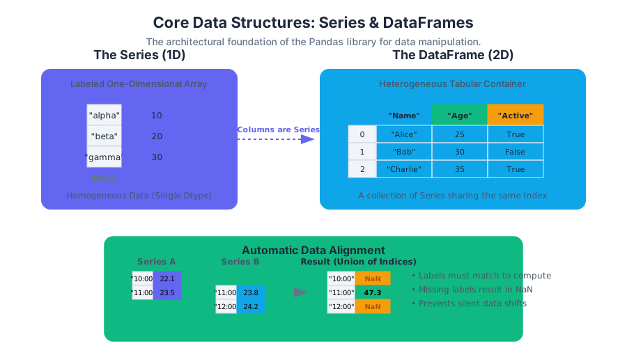
Core Data Structures: Series and DataFrames

Pandas is the foundational library for data manipulation in the Python ecosystem, serving as the bridge between the raw computational power of NumPy and the structured requirements of relational databases and spreadsheets. At its heart, pandas provides two primary data structures: the Series and the DataFrame. These are not merely wrappers around arrays; they are sophisticated objects that integrate data storage, metadata (labels), and automatic alignment logic.

AI_SVGI_SVG## The Series: Labeled One-Dimensional Arrays

A Series is a one-dimensional ndarray with axis labels. While a NumPy array relies on integer-based positional indexing, a Series associates each element with a label, collectively known as the Index. Mathematically, a Series can be viewed as a mapping from a set of labels to a set of values.

Definition: A Series $S$ is a tuple $(V, I, \tau)$ where $V$ is an ordered collection of values, $I$ is an ordered set of unique (or non-unique) labels of the same length as $V$, and $\tau$ is the data type (dtype) of the elements in $V$.

Why the Series Matters

The Series solves the "context loss" problem inherent in standard arrays. In a raw array, the value 32.5 is just a float. In a Series, 32.5 can be associated with the label 2023-10-01, providing immediate temporal or categorical context. This labeling is the mechanism that enables Data Alignment, the most critical feature for handling real-world, "messy" data.

Implementation Mechanics

Internally, a Series stores its data in a contiguous block of memory (usually a NumPy ndarray or a specialized pandas ExtensionArray). The Index is maintained as a separate, highly optimized hash-map-like structure that allows for $O(1)$ lookups of values based on labels.

# Block 1: Low-level implementation and inspection
import numpy as np
import pandas as pd

# Creating a Series with explicit dtype and index
data = np.array([10, 20, 30], dtype=np.int64)
idx = ['alpha', 'beta', 'gamma']
s = pd.Series(data, index=idx, name="GreekData")

# Accessing the underlying memory and index structure
print(f"Dtype: {s.dtype}")
print(f"Values (NumPy): {s.values}")
print(f"Index object: {s.index}")

# Demonstration of label-based vs position-based access
# s.iloc[0] uses the integer offset; s.loc['alpha'] uses the hash map
assert s.iloc[0] == s.loc['alpha']

# Memory usage inspection
print(f"Memory usage (bytes): {s.memory_usage(deep=True)}")

The DataFrame: Heterogeneous Tabular Data

The DataFrame is a two-dimensional, size-mutable, and potentially heterogeneous tabular data structure. It is essentially a container for Series objects, where each Series represents a column. While the Series has one axis (the index), the DataFrame has two: the index (rows) and the columns.

Structural Properties

1. Heterogeneity: Unlike a NumPy matrix, which requires a single dtype for the entire grid, a DataFrame allows each column to have a different dtype (e.g., one column of integers, one of strings, one of datetimes).
2. Dual-Indexing: Operations can be performed along either axis (axis 0 for rows, axis 1 for columns).
3. Dict-like Behavior: A DataFrame can be thought of as a dict of Series objects, where the keys are column names.

Property	Series	DataFrame
Dimensionality	1D	2D
Data Types	Single dtype per Series	Heterogeneous (per-column)
Primary Use	Vectorized sequences	Tabular datasets / SQL-like tables
Mutability	Value mutable	Value and Size mutable
Index	Single Index	Row Index + Column Index

The "Tidy Data" Philosophy

Pandas encourages the "Tidy Data" structure, where:

1. Each variable forms a column.
2. Each observation forms a row.
3. Each type of observational unit forms a table.

AI_DEMOI_DEMO## Data Alignment: The Killer Feature

Data alignment is the process by which pandas automatically matches data from different objects based on their labels during an operation. If you add two Series, pandas does not add them by position (like NumPy); it adds them by matching labels.

The Alignment Algorithm

When an operation is performed between two objects (e.g., $S_1 + S_2$):

1. Union of Indices: Pandas computes the union of the indices of $S_1$ and $S_2$.
2. Reindexing: Both objects are reindexed to this new union index.
3. NaN Injection: Labels present in one object but not the other are filled with NaN (Not a Number).
4. Vectorized Operation: The operation is performed on the aligned values.

% Block 2: Mathematical Derivation of Alignment
Let S_1 = { (l_i, v_i) } and S_2 = { (k_j, w_j) }
The result R = S_1 \oplus S_2 is defined as:

Index(R) = I_{S1} \cup I_{S2}

Value(R)_m = 
\begin{cases} 
v_m \oplus w_m & \text{if } m \in I_{S1} \cap I_{S2} \\
\text{NaN} & \text{otherwise}
\end{cases}

Worked Example of Alignment

Imagine two sensors recording temperatures at different times. Sensor A records at 10:00 and 11:00. Sensor B records at 11:00 and 12:00.

# Block 3: Real-world usage - Alignment in Action
s_a = pd.Series([22.1, 23.5], index=['10:00', '11:00'])
s_b = pd.Series([23.8, 24.2], index=['11:00', '12:00'])

# Adding these Series aligns them by timestamp
avg_temp = (s_a + s_b) / 2

print(avg_temp)
# Output:
# 10:00     NaN
# 11:00    23.65
# 12:00     NaN
# dtype: float64

This behavior prevents "silent errors" where data from different time points or categories are accidentally combined due to shifts in the data array.

Index Labels and Selection Logic

The Index is the most misunderstood component of pandas. It is not just a row counter; it is an immutable array acting as a metadata layer. Pandas provides several ways to access data, primarily through loc (label-based) and iloc (integer-position-based).

Indexing Methods Comparison

Method	Access Type	Logic	Use Case
.loc[]	Label-based	Strict matching of index/column labels.	Production code, filtering by ID/Date.
.iloc[]	Position-based	0-based integer indexing (like Python lists).	Programmatic loops, train/test splits.
.at[]	Label-based	Fast access for a single scalar value.	High-performance single-cell updates.
[]	Hybrid	Column selection or slicing.	Quick interactive exploration.

Common Pitfall: The SettingWithCopyWarning

A common error for senior engineers is attempting to modify a subset of a DataFrame: df[df['A'] > 5]['B'] = 10. This often fails because df[df['A'] > 5] might return a view or a copy. Pandas cannot guarantee that the assignment will propagate back to the original DataFrame. The correct approach is always to use .loc: df.loc[df['A'] > 5, 'B'] = 10.

Handling Missing Data (NaN)

Pandas was one of the first libraries to treat missing data as a first-class citizen. It primarily uses np.nan (from the IEEE 754 floating-point specification) to represent missing values.

The Nature of NaN

• NaN is a float. Therefore, an integer column containing a NaN will be automatically cast to float64.
• NaN != NaN. This is a standard floating-point rule. To detect missing values, one must use pd.isna() or pd.isnull().
• Propagation: In arithmetic, 5 + NaN = NaN. In aggregations (like .sum()), pandas defaults to ignoring NaN (treating it as 0 or simply skipping it), which differs from NumPy's default behavior.

Strategies for Missing Data

Strategy	Method	Description
Detection	isna() / notna()	Returns a boolean mask of missing values.
Removal	dropna()	Removes rows or columns containing missing values.
Imputation	fillna()	Replaces NaN with a scalar or a calculated value (mean/median).
Interpolation	interpolate()	Fills NaN using linear, polynomial, or time-based logic.

# Block 4: Edge cases and Nullable Types
# Traditional behavior: Integer column becomes float due to NaN
s_int = pd.Series([1, 2, None], dtype=object) # Forced to object or float
print(f"Traditional dtype with None: {pd.Series([1, 2, np.nan]).dtype}")

# Modern Pandas (1.0+): Nullable Integer Types
# Using the capital 'I' Integer dtype allows NaNs without casting to float
s_nullable = pd.Series([1, 2, None], dtype="Int64")
print(f"Nullable Integer dtype: {s_nullable.dtype}")
print(f"Is element 2 null? {s_nullable.isna()[2]}")

# Performance comparison: Vectorized fillna vs manual loop
# df.fillna(0) is orders of magnitude faster than iterating rows

Advanced Concept: MultiIndex (Hierarchical Indexing)

While DataFrames are 2D, the MultiIndex allows pandas to represent higher-dimensional data within a 2D structure. This is essentially "nesting" indices.

Why MultiIndex?

It allows for sophisticated "group-by" operations and data reshaping (pivoting). For example, a dataset tracking "Sales" across "Year" and "Region" can have a MultiIndex of ['Year', 'Region'].

Mechanics

A MultiIndex is stored as a list of levels (the unique labels for each level) and codes (integers mapping each position to a level label). This representation is extremely memory-efficient.

# Block 5: DevOps/Environment Setup for Pandas Performance
# High-performance pandas often requires specific C-extensions and engines
# Install pandas with performance extras:
pip install "pandas[performance, excel, parquet]"

# For faster I/O, ensure 'pyarrow' or 'fastparquet' is available
# For faster expression evaluation, 'numexpr' is recommended
pip install pyarrow numexpr

# Set environment variable to use the 'PyArrow' backed strings (Pandas 3.0+ default)
export PANDAS_USE_PYARROW=1

Summary of Best Practices

1. Vectorization over Loops: Never iterate over a DataFrame with for index, row in df.iterrows() unless absolutely necessary. Use vectorized Series operations.
2. Explicit Indexing: Use .loc and .iloc to avoid ambiguity and SettingWithCopy warnings.
3. Dtype Management: Downcast numeric types (float64 to float32) and use category dtypes for low-cardinality strings to save up to 90% memory.
4. Alignment Awareness: Always check indices before joining or adding Series to ensure you aren't creating unintended NaN values.

AI_STUDY_GUIDEI_STUDY_GUIDE### Further Reading

• The "Tidy Data" paper by Hadley Wickham.
• Pandas Internals: The BlockManager vs. the new ArrayManager.
• IEEE 754 Floating-Point Standard and its implications for data science.

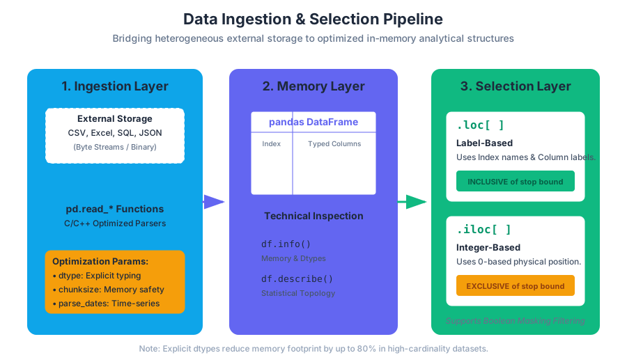
Data Ingestion and Selection

Data rarely originates within the sterile environment of a Python script. In the lifecycle of a data engineering pipeline, the Ingestion Layer serves as the critical interface between heterogeneous external storage systems—ranging from legacy flat files to enterprise-grade distributed databases—and the structured, in-memory representation required for analytical computation. Once data is resident in memory (typically as a pandas DataFrame), the Selection Layer provides the mechanism for dimensionality reduction, filtering, and feature isolation.

Mastering these two phases is not merely a matter of syntax; it is about understanding the memory layout of tabular data and the performance implications of how we access it.

AI_SVGI_SVG## 1. The Ingestion Layer: Bridging Storage and Memory

The ingestion process in pandas is governed by a suite of read_* functions. These are highly optimized wrappers around lower-level parsers (often written in C or C++) designed to convert byte streams into typed NumPy arrays.

1.1 The CSV Standard and read_csv

The Comma-Separated Values (CSV) format is the lingua franca of data exchange. Despite its ubiquity, it lacks a formal schema, making the read_csv function one of the most complex and parameter-rich tools in the pandas library.

Definition: Schema Inference The process by which a parser scans a subset of a file (the "sniff" phase) to automatically determine the data type (dtype) of each column. While convenient, schema inference is computationally expensive and prone to errors in large datasets with sparse values.

Parameter	Type	Purpose	Performance Impact
filepath_or_buffer	str/path/buffer	Source of the data (local path, URL, or S3/GCS)	High (I/O bound)
sep	str	Delimiter (default ,). Can use regex for complex formats.	Low
dtype	dict	Explicitly defines column types (e.g., {'id': np.int32})	High (Reduces memory & prevents re-scanning)
parse_dates	list/bool	Converts columns to datetime64[ns] objects	Medium
chunksize	int	Returns an iterable TextFileReader for out-of-memory processing	Critical for Big Data
low_memory	bool	Internally process file in chunks to lower memory usage (C engine only)	Medium

1.2 The Excel Ecosystem and read_excel

Unlike CSVs, Excel files (.xlsx, .xlsb) are binary formats (OpenXML) that contain metadata, multiple sheets, and formatting. read_excel relies on engines like openpyxl or pyxlsb to decode these structures.

1.3 Implementation: High-Performance Ingestion

The following example demonstrates a production-grade ingestion pattern using explicit dtypes and date parsing to minimize the memory footprint.

import pandas as pd
import numpy as np

# Defining a schema for ingestion to optimize memory and ensure type safety
schema = {
    'transaction_id': 'int64',
    'customer_id': 'category',  # Categorical saves massive memory for low-cardinality strings
    'amount': 'float32',        # float32 is often sufficient and uses 50% less RAM than float64
    'status': 'category'
}

def ingest_financial_data(file_path: str):
    """
    Ingests large-scale CSV data with optimized memory mapping.
    """
    try:
        # Using chunksize for a memory-efficient stream
        reader = pd.read_csv(
            file_path,
            sep=',',
            dtype=schema,
            parse_dates=['timestamp'],
            infer_datetime_format=True,
            engine='c', # Use the optimized C engine
            low_memory=False
        )
        return reader
    except FileNotFoundError as e:
        print(f"I/O Error: {e}")
        return None

# Execution
# df = ingest_financial_data("large_ledger.csv")

2. Data Inspection: The Technical Summary

Before selection can occur, an engineer must understand the topology of the data. This is achieved through inspection methods that reveal the "technical metadata" of the object.

• df.head(n) / df.tail(n): Returns the first or last $n$ rows. Essential for visual verification of parsing success.
• df.info(): The most critical diagnostic tool. It displays the Index, Column names, Non-Null Count, and Dtype. Most importantly, it provides the memory usage estimate.
• df.describe(): Generates descriptive statistics (mean, std, quartiles) for numerical columns.

AI_DEMOI_DEMO## 3. The Mechanics of Selection: loc vs iloc

The most common source of bugs in pandas code is the confusion between label-based and position-based indexing. Pandas provides two primary accessors to resolve this ambiguity.

3.1 loc: Label-Based Selection

The .loc accessor is used when you want to access data based on the Index label or Column name. It is inclusive of both the start and the stop bounds.

Theorem: Label Alignment Pandas operations are intrinsically aligned by label. When using .loc, the system searches the hash map of the index to find the corresponding physical memory address.

3.2 iloc: Integer-Based Selection

The .iloc accessor is strictly positional. It treats the DataFrame like a standard NumPy array or Python list, using 0-based indexing. Unlike .loc, it follows standard Python slicing conventions (inclusive of start, exclusive of stop).

3.3 Comparative Analysis

Feature	.loc	.iloc
Primary Input	Index Labels / Column Names	Integer Positions (0 to length-1)
Slicing Behavior	Inclusive of stop: ['a':'c'] includes 'c'	Exclusive of stop: [0:2] excludes index 2
Boolean Arrays	Accepted	Accepted (but less common)
Use Case	Semantic queries ("Get 'Sales' for 'March'")	Algorithmic queries ("Get the first 10 rows")

3.4 Logic of Selection (Pseudocode)

Understanding how pandas resolves these calls internally can be visualized as a lookup strategy:

FUNCTION SelectData(Object, Key, Mode):
    IF Mode == "LABEL":
        # Search the Index Hash Table
        PhysicalIndex = Object.Index.Map.Get(Key)
        RETURN MemoryBlock[PhysicalIndex]
    
    ELSE IF Mode == "POSITION":
        # Direct Offset Calculation
        IF Key < 0 OR Key >= Object.Length:
            THROW IndexError
        RETURN MemoryBlock[Key]
END FUNCTION

4. Boolean Indexing: The Declarative Query

Boolean indexing allows for the selection of data based on the values within the DataFrame rather than their coordinates. This is a vectorized operation, meaning the condition is applied to every element in a column simultaneously.

4.1 Logical Operators

When combining multiple conditions, pandas requires the use of bitwise operators rather than Python's and/or keywords. This is because bitwise operators are overloaded to perform element-wise comparisons on arrays.

• & (AND): Both conditions must be true.
• | (OR): At least one condition must be true.
• ~ (NOT): Inverts the boolean mask.

4.2 Vectorized Filtering with isin() and notna()

For more complex filtering, pandas provides specialized methods that are significantly faster than manual loops.

• isin([list]): Returns a boolean mask where True indicates the value exists in the provided list. This is essentially a vectorized SQL IN clause.
• notna(): Returns a mask identifying non-missing values. This is crucial for data cleaning pipelines where NaN (Not a Number) values would break downstream mathematical models.

4.3 Real-World Usage Example

Consider a dataset of Titanic passengers. We want to find adult females who survived, excluding those with missing age data, and who traveled in 1st or 2nd class.

# Example of a CLI-based data exploration workflow
# 1. Download data
curl -O https://raw.githubusercontent.com/pandas-dev/pandas/main/doc/data/titanic.csv

# 2. Run a python snippet to perform complex selection
python3 -c "
import pandas as pd
df = pd.read_csv('titanic.csv')

# Complex Boolean Indexing
# Criteria: Female, Survived, Age known, Class in [1, 2]
mask = (
    (df['Sex'] == 'female') & 
    (df['Survived'] == 1) & 
    (df['Age'].notna()) & 
    (df['Pclass'].isin([1, 2]))
)

subset = df.loc[mask, ['Name', 'Age', 'Pclass']]
print(f'Found {len(subset)} passengers matching criteria.')
print(subset.head())
"

5. Advanced Selection Patterns

5.1 Simultaneous Row and Column Selection

One of the most powerful features of .loc and .iloc is the ability to slice both axes at once. The syntax is df.loc[row_indexer, column_indexer].

# Select rows 10 through 20, and only columns 'Age' through 'Fare'
# Note: .loc is inclusive of 'Fare'
refined_view = df.loc[10:20, 'Age':'Fare']

# Select the first 5 rows and the first 3 columns by position
fast_slice = df.iloc[:5, :3]

5.2 The notna() and isna() Duality

Handling missing data is a prerequisite for any selection. Missing values in pandas are typically represented by np.nan (for floats/objects) or pd.NA (for nullable integers).

\text{Mask}_{i} = 
\begin{cases} 
1 & \text{if } x_i \neq \text{NaN} \\
0 & \text{if } x_i = \text{NaN}
\end{cases}
\quad \forall x \in \text{Column}

The notna() method generates this mask, allowing for the exclusion of incomplete records: clean_df = df[df['email_address'].notna()]

6. Common Pitfalls and Performance Bottlenecks

6.1 The SettingWithCopyWarning

This is the most frequent warning encountered by beginners. It occurs when you attempt to modify a subset of a DataFrame that pandas cannot determine is a view or a copy.

• Bad: df[df['A'] > 2]['B'] = 0 (Chained indexing)
• Good: df.loc[df['A'] > 2, 'B'] = 0 (Single-step access)

6.2 Memory Inefficiency in Ingestion

Loading a 1GB CSV into pandas can often result in a 4GB+ DataFrame in memory. This is because pandas defaults to 64-bit types (int64, float64).

Data Type	Memory (per value)	Range
int8	1 byte	-128 to 127
int64	8 bytes	$\pm 9 \times 10^{18}$
float32	4 bytes	Standard precision
category	Variable	Optimized for repeating strings

Pro Tip: Always use df.info(memory_usage='deep') to get the true memory footprint, as object-type columns (strings) are otherwise not fully accounted for.

AI_STUDY_GUIDEI_STUDY_GUIDE--

Study Guide: Data Ingestion and Selection

Core Concepts to Master

1. The I/O Pipeline: Understand that read_csv is a complex parser. Know when to use dtype to save memory and parse_dates to enable time-series functionality.
2. The Indexing Duality:
   • .loc = Labels (Semantic).
   • .iloc = Positions (Numerical).
3. Boolean Logic: Master the use of &, |, and ~. Remember that parentheses are mandatory around conditions due to operator precedence.
4. Vectorized Filters: Prefer isin() over multiple == OR statements. Use notna() to filter out null values before computation.

Practical Exercises

• Exercise 1: Load a dataset and use df.info() to identify columns that could be downcast from int64 to int8 or converted to category.
• Exercise 2: Write a selection statement that finds all rows where a specific numerical column is above the mean AND a categorical column is in a specific list of values.
• Exercise 3: Compare the output of df.loc[0:5] and df.iloc[0:5] on a DataFrame where the index has been shuffled. Observe how .loc follows the labels while .iloc follows the order.

Technical Vocabulary

• Vectorization: Performing operations on entire arrays rather than individual elements.
• Chained Indexing: The practice of using multiple sets of brackets (e.g., df[][]), which leads to unpredictable behavior.
• Downcasting: Converting a data type to a lower-bit representation to save memory.
• Label Alignment: The internal mechanism that ensures data is matched based on index labels during operations.

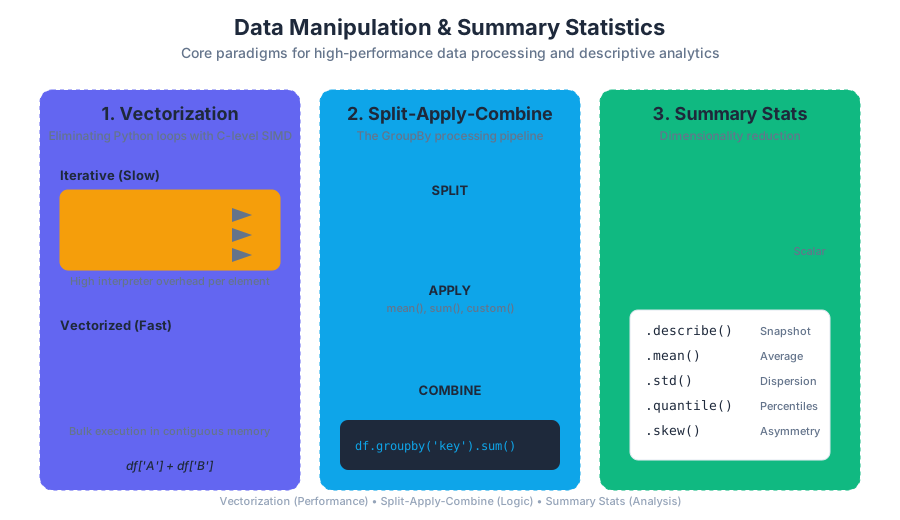
Data Manipulation and Summary Statistics

In the realm of computational data science, the transition from raw, unstructured observations to actionable insights is mediated by two fundamental capabilities: the ability to perform high-performance bulk operations and the ability to reduce high-dimensional data into meaningful summaries. This section explores the mechanics of Vectorization, the conceptual framework of Split-Apply-Combine, and the rigorous application of Summary Statistics within the pandas ecosystem.

AI_SVGI_SVG## Vectorization: The Engine of Performance

At the heart of pandas lies the principle of Vectorization. In traditional imperative programming, operations on a collection of items are typically handled via explicit loops (e.g., for or while). Vectorization replaces these explicit loops with "array-oriented" operations that occur at the compiled C and Cython levels.

What it is

Vectorization is the process of executing an operation on an entire array (or Series) at once, rather than iterating through individual elements. Mathematically, if we have two vectors $\mathbf{a}$ and $\mathbf{b}$ of length $n$, a vectorized addition $\mathbf{c} = \mathbf{a} + \mathbf{b}$ computes $c_i = a_i + b_i$ for all $i \in {1, \dots, n}$ in a single conceptual step.

Why it matters

Python is an interpreted language, and the overhead of the Python interpreter—type checking, dynamic dispatch, and object creation—within a loop can be orders of magnitude slower than the actual arithmetic operation. Vectorization delegates the loop to highly optimized C or Fortran code (via NumPy), leveraging SIMD (Single Instruction, Multiple Data) instructions at the CPU level.

How it works

When you execute df['A'] + df['B'], pandas does not call the Python + operator $n$ times. Instead, it identifies the underlying memory buffers (NumPy arrays) and passes pointers to these buffers to a pre-compiled C routine. This routine iterates through the contiguous memory blocks, minimizing cache misses and maximizing throughput.

Feature	Iterative (Loops)	Vectorized (Pandas/NumPy)
Execution Speed	Slow (High Python overhead)	Fast (C-level execution)
Code Readability	Verbose, boilerplate-heavy	Concise, mathematical
Memory Access	Frequent pointer chasing	Contiguous memory blocks
Type Safety	Checked at every iteration	Checked once per array

import pandas as pd
import numpy as np
import time

# Generating a dataset with 10 million rows
n = 10_000_000
df = pd.DataFrame({
    'price': np.random.uniform(10, 100, size=n),
    'quantity': np.random.randint(1, 10, size=n)
})

# 1. THE SLOW WAY: Manual Iteration (Anti-pattern)
start = time.time()
total_loop = []
for i in range(len(df)):
    total_loop.append(df.iloc[i]['price'] * df.iloc[i]['quantity'])
end = time.time()
print(f"Loop time: {end - start:.4f} seconds")

# 2. THE FAST WAY: Vectorization
start = time.time()
df['total'] = df['price'] * df['quantity']
end = time.time()
print(f"Vectorized time: {end - start:.4f} seconds")

AI_DEMOI_DEMO## Summary Statistics: Descriptive Analytics

Summary statistics are the primary tools used to describe the distribution, central tendency, and dispersion of a dataset. In pandas, these are implemented as reducing methods that collapse a dimension of a DataFrame or Series into a single scalar value.

The describe() Method

The most comprehensive entry point for summary statistics is the .describe() method. It provides a diagnostic "snapshot" of the data. For numerical data, it returns:

1. Count: Number of non-null observations.
2. Mean: The arithmetic average.
3. Std: Standard deviation (a measure of spread).
4. Min/Max: The range boundaries.
5. Percentiles: The 25th, 50th (median), and 75th percentiles.

Mathematical Foundations

Pandas uses the "N-1" convention for sample standard deviation by default (Bessel's correction), which provides an unbiased estimate of the population variance from a sample.

s = \sqrt{\frac{\sum_{i=1}^{n} (x_i - \bar{x})^2}{n - 1}}

Where:

• $x_i$ is an individual observation.
• $\bar{x}$ is the sample mean.
• $n$ is the number of observations.

Common Statistical Methods

Method	Description	SQL Equivalent
.mean()	Arithmetic mean of values	AVG()
.median()	Median (50th percentile)	PERCENTILE_CONT(0.5)
.std()	Sample standard deviation	STDEV()
.var()	Unbiased variance	VAR()
.skew()	Sample skewness (3rd moment)	N/A (Standard)
.kurt()	Sample kurtosis (4th moment)	N/A (Standard)
.quantile(q)	Value at quantile $q$	PERCENTILE_DISC(q)

The Split-Apply-Combine Paradigm

The most powerful pattern in data manipulation is Split-Apply-Combine, a term coined by Hadley Wickham. It describes a strategy where a large problem is broken down into manageable pieces, operated upon, and then reassembled.

Definition: Split-Apply-Combine is a data processing strategy where a dataset is partitioned into groups (Split), a function is executed on each group independently (Apply), and the results are concatenated into a new data structure (Combine).

1. Split

The groupby() function is the primary mechanism for splitting. It creates a GroupBy object, which is a "lazy" representation of the data. No computation happens during the split phase; pandas simply maps the index labels to group identifiers.

2. Apply

Once the data is split, you apply a function. There are three main categories of application:

• Aggregation: Reduces each group to a single value (e.g., sum, mean, count).
• Transformation: Performs a group-specific computation but returns an object with the same shape as the original (e.g., standardizing data within a group).
• Filtration: Discards entire groups based on a boolean condition (e.g., removing groups with fewer than 100 observations).

3. Combine

Pandas automatically handles the reassembly of the results. If the apply step returns a scalar per group, the result is a Series (or DataFrame if multiple columns were aggregated) with the group keys as the index.

/* 
A conceptual representation of Split-Apply-Combine in SQL 
This shows how the 'Split' (GROUP BY) and 'Apply' (SUM) 
work together to 'Combine' into a result set.
*/

SELECT 
    department_id, 
    SUM(salary) AS total_payroll,
    AVG(salary) AS avg_salary
FROM 
    employees
WHERE 
    hire_date > '2020-01-01'
GROUP BY 
    department_id
HAVING 
    COUNT(*) > 5;

Groupby Mechanics and Syntax

The syntax for groupby in pandas is highly flexible, allowing for grouping by column names, levels of a MultiIndex, or even external arrays.

Aggregation via .agg()

While you can call .sum() directly on a GroupBy object, the .agg() (or .aggregate()) method allows for much more granular control, such as applying different functions to different columns.

Transformation via .transform()

Transformation is often misunderstood. Unlike aggregation, which reduces the number of rows, transformation preserves the original index. This is critical for operations like "percent of group total" or "group-wise imputation."

# Real-world usage: Financial Data Normalization
import pandas as pd

data = {
    'Sector': ['Tech', 'Tech', 'Energy', 'Energy', 'Tech', 'Retail'],
    'Ticker': ['AAPL', 'MSFT', 'XOM', 'CVX', 'NVDA', 'WMT'],
    'Price': [150, 250, 80, 120, 400, 140],
    'MarketCap': [2.5, 2.2, 0.4, 0.3, 1.1, 0.5] # In Trillions
}
df = pd.DataFrame(data)

# 1. Aggregation: What is the total market cap per sector?
sector_totals = df.groupby('Sector')['MarketCap'].sum()

# 2. Transformation: Z-Score of price within each sector
# Formula: (x - mean) / std
z_score = lambda x: (x - x.mean()) / x.std()
df['Sector_Z_Score'] = df.groupby('Sector')['Price'].transform(z_score)

# 3. Filtration: Keep only sectors with more than 1 ticker
large_sectors = df.groupby('Sector').filter(lambda x: len(x) > 1)

Renaming and Metadata Management

Data manipulation often results in cryptic column names (e.g., Price_x, Price_y) or uninformative index labels. Renaming is the process of updating the metadata of the DataFrame to maintain clarity and ensure that downstream code remains readable.

The rename Method

The .rename() method is the standard tool for this. It accepts a dictionary-like "mapper" or a function.

• Axis-based: df.rename(columns={'old_name': 'new_name'})
• Functional: df.rename(columns=str.lower) (converts all columns to lowercase)

In-place vs. Copy

By default, pandas operations return a copy of the data. While an inplace=True parameter exists for many methods, it is generally discouraged in modern pandas (and deprecated in some contexts) because it can lead to SettingWithCopyWarning and prevents method chaining.

Approach	Syntax	Best Use Case
Dictionary Mapper	df.rename(columns={'A': 'Alpha'})	Specific, targeted changes
String Methods	df.rename(columns=str.strip)	Cleaning whitespace/formatting
Direct Assignment	df.columns = ['New1', 'New2']	Renaming all columns at once
Set Index	df.set_index('Date')	Promoting a column to the index

Value Counts: Categorical Frequency

For categorical data, the .value_counts() method is the most efficient way to understand the distribution of classes. It returns a Series where the index is the unique values and the values are the frequencies, sorted in descending order.

Normalization

By setting normalize=True, the method returns relative frequencies (proportions) instead of raw counts. This is essential for comparing datasets of different sizes.

# Using the command line to inspect a CSV before pandas processing
# This is a common first step for senior engineers to check 
# categorical distribution (similar to value_counts)

# Count unique values in the 2nd column (Sector) of a CSV
cut -d',' -f2 data.csv | sort | uniq -c | sort -nr

# Output looks like:
#   3 Tech
#   2 Energy
#   1 Retail

Common Pitfalls and Best Practices

1. The "Loop" Temptation

New users often fall back on df.iterrows(). While it feels familiar, it is almost always the wrong choice. iterrows() returns a Series for each row, which involves a massive amount of type conversion and object overhead. Solution: Always look for a vectorized alternative or use .apply() (though even .apply() is just a fancy loop).

2. Chained Indexing

df[df['A'] > 5]['B'] = 10 often triggers a SettingWithCopyWarning. This happens because pandas cannot guarantee if df[df['A'] > 5] is a view of the original memory or a new copy. Solution: Use .loc for assignment: df.loc[df['A'] > 5, 'B'] = 10.

3. Memory Management in Groupby

Grouping by a high-cardinality column (e.g., a unique UserID in a billion-row dataset) can consume vast amounts of RAM because pandas creates an entry for every unique key in the resulting index. Solution: Ensure the grouping column is of the category dtype to reduce memory footprint.

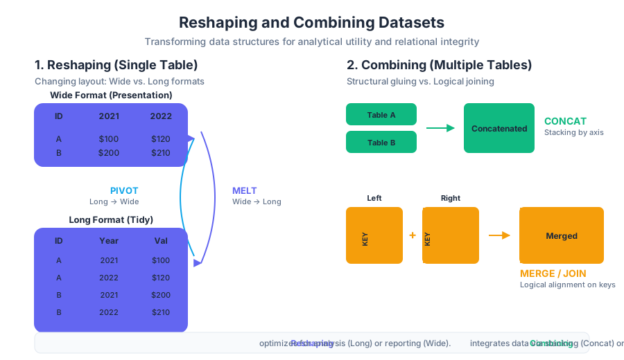
Reshaping and Combining Datasets

In the lifecycle of data engineering and analysis, raw data rarely arrives in a format ready for immediate consumption. It is often fragmented across disparate sources—SQL databases, CSV logs, or JSON API responses—and structured in ways that prioritize storage efficiency or capture convenience over analytical utility. Reshaping and combining are the fundamental operations used to transform these "wild" datasets into "tidy" structures suitable for machine learning, statistical modeling, and visualization.

AI_SVGI_SVGt its core, reshaping is about changing the layout of a single table to better represent the relationship between variables and observations. Combining is about the integration of multiple tables into a unified whole, ensuring that relational integrity is maintained across different axes of information. Mastering these operations requires an understanding of both the algebraic properties of relational joins and the memory-management implications of data alignment.

The Taxonomy of Data Shapes: Long vs. Wide

Before applying transformations, one must identify the current and target "shape" of the data. In the context of tabular data, we categorize structures into two primary formats: Long (also known as "stacked" or "tidy") and Wide (also known as "unstacked" or "presentation" format).

Definition: Tidy Data A dataset is considered "tidy" when:

1. Each variable forms a column.
2. Each observation forms a row.
3. Each type of observational unit forms a table.

Comparison of Data Formats

Feature	Wide Format	Long Format
Structure	Variables are spread across multiple columns (e.g., Year_2020, Year_2021).	Variables are stored in a single "Key" column with values in a "Value" column.
Readability	High for humans; easy to compare values side-by-side.	Low for humans; repetitive identifiers.
Analysis	Difficult for group-by operations or time-series modeling.	Ideal for seaborn plotting, scikit-learn modeling, and SQL-like aggregations.
Scalability	Adding a new category requires adding a new column (schema change).	Adding a new category requires adding new rows (no schema change).
Memory	Often more compact for sparse data.	Can be memory-intensive due to repeated index/ID labels.

Reshaping Mechanics: Pivot and Melt

Reshaping is the process of rotating the data's axes. In the Python/Pandas ecosystem, this is primarily handled by pivot, pivot_table, and melt.

Pivot: From Long to Wide

The pivot operation takes unique values from one column and turns them into column headers for a new DataFrame. This is essentially a "de-normalization" step used for reporting or creating correlation matrices.

• Index: The column(s) to use as the new row labels.
• Columns: The column whose unique values will become the new column headers.
• Values: The column(s) whose values will fill the new table cells.

If your data has duplicate entries for the same index/column pair, pivot will fail. In such cases, pivot_table is required, as it allows for an aggregation function (like mean, sum, or count) to resolve collisions.

Melt: From Wide to Long

The melt operation is the inverse of pivot. It "unpivots" a DataFrame from a wide format to a long format, which is often a prerequisite for advanced data cleaning.

• id_vars: Columns that should remain as identifiers (not melted).
• value_vars: Columns to be unpivoted (if not specified, uses all columns not in id_vars).
• var_name: Name for the new "variable" column.
• value_name: Name for the new "value" column.

import pandas as pd
import numpy as np

# Low-level implementation of a Pivot-like transformation using pure Python 
# to demonstrate the underlying logic of coordinate mapping.
def manual_pivot(data, index_col, columns_col, values_col):
    """
    Simulates the logic of pd.pivot: 
    Maps (row_id, col_id) pairs to a 2D grid.
    """
    # Identify unique coordinates
    unique_indices = sorted(list(set(row[index_col] for row in data)))
    unique_columns = sorted(list(set(row[columns_col] for row in data)))
    
    # Create mapping for O(1) lookup
    idx_map = {val: i for i, val in enumerate(unique_indices)}
    col_map = {val: i for i, val in enumerate(unique_columns)}
    
    # Initialize an empty matrix (NaN-filled)
    matrix = np.full((len(unique_indices), len(unique_columns)), np.nan)
    
    # Fill the matrix
    for entry in data:
        r = idx_map[entry[index_col]]
        c = col_map[entry[columns_col]]
        matrix[r, c] = entry[values_col]
        
    return matrix, unique_indices, unique_columns

# Example usage with raw dictionary data
raw_data = [
    {'city': 'NYC', 'date': '2023-01-01', 'temp': 32},
    {'city': 'NYC', 'date': '2023-01-02', 'temp': 35},
    {'city': 'LA', 'date': '2023-01-01', 'temp': 70},
    {'city': 'LA', 'date': '2023-01-02', 'temp': 72},
]

pivoted, rows, cols = manual_pivot(raw_data, 'date', 'city', 'temp')
print(f"Columns: {cols}\nRows: {rows}\nMatrix:\n{pivoted}")

AI_DEMOI_DEMO## Combining Datasets: Concatenation and Merging

While reshaping deals with the internal structure of a single dataset, combining deals with the relationship between multiple datasets. We distinguish between Concatenation (structural gluing) and Merging (logical joining).

Concatenation (pd.concat)

Concatenation is the process of "stacking" DataFrames along a particular axis.

• Axis 0 (Rows): Stacking tables vertically. This is common when you have monthly logs (Jan, Feb, Mar) and want a single year-to-date table.
• Axis 1 (Columns): Aligning tables horizontally based on their index.

Concatenation is primarily a structural operation. It does not look at the content of the columns to find matches; it relies on the alignment of labels (indexes or column names).

Merging (pd.merge)

Merging is a relational operation, analogous to SQL JOINs. It combines tables based on the values of one or more "keys."

The Join Theorem Given two sets $L$ (Left) and $R$ (Right), a Join operation $L \bowtie R$ produces a set of tuples $(l, r)$ such that $l \in L, r \in R$ and a predicate $P(l, r)$ is satisfied (usually $l.key = r.key$).

Join Types and Logic

Join Type	Pandas Argument	SQL Equivalent	Result Description
Inner	how='inner'	INNER JOIN	Only keys present in both tables are kept.
Left	how='left'	LEFT OUTER JOIN	All keys from the left table are kept; right values are NaN if no match.
Right	how='right'	RIGHT OUTER JOIN	All keys from the right table are kept; left values are NaN if no match.
Outer	how='outer'	FULL OUTER JOIN	All keys from both tables are kept; missing values are filled with NaN.
Cross	how='cross'	CROSS JOIN	Cartesian product: every row of left paired with every row of right.

\begin{aligned}
&\text{Let } A = \{ (k_1, v_1), (k_2, v_2) \} \text{ and } B = \{ (k_1, w_1), (k_3, w_3) \} \\
&\text{Inner Join: } A \cap_k B = \{ (k_1, v_1, w_1) \} \\
&\text{Left Join: } A \cup_k B_{left} = \{ (k_1, v_1, w_1), (k_2, v_2, \text{NaN}) \} \\
&\text{Outer Join: } A \cup_k B = \{ (k_1, v_1, w_1), (k_2, v_2, \text{NaN}), (k_3, \text{NaN}, w_3) \}
\end{aligned}

Merge Implementation in Practice

The power of pd.merge lies in its flexibility regarding key names. If the keys are named differently in each table, we use left_on and right_on.

-- SQL Representation of a complex merge
-- This logic is what pd.merge(df1, df2, left_on='user_id', right_on='id', how='left') executes
SELECT 
    df1.user_id, 
    df1.purchase_amount, 
    df2.user_name, 
    df2.signup_date
FROM 
    transactions AS df1
LEFT JOIN 
    users AS df2
ON 
    df1.user_id = df2.id;

Advanced Reshaping: Stack and Unstack

For datasets with Hierarchical Indexing (MultiIndex), Pandas provides the stack() and unstack() methods. These are specialized versions of pivot/melt designed for multi-level labels.

• Stack: "Compresses" a level in the DataFrame's columns to produce a multi-level index (moving from wide to long).
• Unstack: "Expands" a level in the DataFrame's index into the column axis (moving from long to wide).

Comparison: Pivot vs. Stack

Operation	Best Used When...	Handling of Missing Data
Pivot	You want to specify exactly which columns become the new index/columns.	Leaves NaN where no match exists.
Stack	You have a MultiIndex and want to rotate a specific level.	Automatically drops NaN values by default (dropna=True).

Common Pitfalls and Performance Considerations

1. The Cartesian Product Explosion

When merging on keys that are not unique in both tables, the resulting DataFrame can grow exponentially. If Table A has 1,000 instances of key=1 and Table B has 1,000 instances of key=1, an inner join will produce 1,000,000 rows for that key alone.

• Fix: Always check for duplicates in your keys using df.duplicated(subset=['key']).any() before merging.

2. Loss of Integer Dtypes (The NaN Problem)

In Pandas (prior to version 1.0), the standard integer type (int64) did not support NaN. If a merge or pivot introduced missing values, the entire column would be silently cast to float64.

• Fix: Use the nullable integer type Int64 (capital 'I') or ensure data completeness before joining.

3. Memory Fragmentation

Repeatedly concatenating DataFrames in a loop (e.g., for file in files: df = pd.concat([df, pd.read_csv(file)])) is an $O(N^2)$ operation because Pandas creates a new copy of the entire dataset at every iteration.

• Fix: Collect all DataFrames in a list and call pd.concat once.

# Performance Tip: Inspecting keys before a merge using CLI tools
# This helps identify if 'user_id' is a viable join key without loading 10GB into RAM.

# Count unique keys in a CSV
cut -d',' -f1 large_data.csv | sort | uniq -c | sort -nr | head -n 10

# Check for null keys in the join column
awk -F',' '$1 == "" {print "Empty key found at line " NR}' large_data.csv

Real-World Workflow: The "Reshape-Combine" Pipeline

Often, a data task requires a sequence of these operations. Consider a scenario where you have weather data in multiple CSVs (one per city) in a wide format, and you need to join it with a central "City Metadata" table.

1. Read & Concat: Load all city CSVs and pd.concat them into one master wide table.
2. Melt: Convert the wide table (columns like Jan, Feb, Mar) into a long table (Month, Temperature).
3. Merge: Join the long table with the City_Metadata table on the City_ID key.
4. Pivot Table: Create a final summary report showing average temperature by Region (from metadata) and Season.

AI_STUDY_GUIDEI_STUDY_GUIDE### Summary Table of Operations

Goal	Primary Method	Key Parameter
Stack rows vertically	pd.concat([df1, df2])	axis=0
Join on shared values	pd.merge(df1, df2)	on='key_col'
Turn rows into columns	df.pivot()	columns='col_to_rotate'
Turn columns into rows	df.melt()	id_vars=['keep_cols']
Aggregate while pivoting	df.pivot_table()	aggfunc='mean'
Rotate MultiIndex levels	df.stack() / df.unstack()	level=-1

Specialized Data: Time Series and Text

In the landscape of data science, tabular data is rarely composed solely of integers and floats. Two of the most semantically rich—and computationally challenging—data types are Temporal (Time Series) and Textual (Strings). While a standard Python list or a NumPy array treats these as generic objects, pandas elevates them to first-class citizens through specialized internal engines and "accessor" objects.

This section explores the mechanics of the DatetimeIndex, the temporal arithmetic of Timedelta, the frequency-based logic of Resampling, and the vectorized power of the str and dt accessors. Understanding these tools is the difference between writing slow, brittle for loops and writing performant, idiomatic data pipelines.

The Temporal Backbone: DatetimeIndex and pd.to_datetime

At the heart of pandas' time-series capabilities lies the DatetimeIndex. Unlike a standard integer index, a DatetimeIndex is optimized for chronological slicing, frequency awareness, and timezone localization.

What it is

A DatetimeIndex is a specialized index of Timestamp objects. Internally, pandas stores these timestamps as 64-bit integers representing nanoseconds since the Unix Epoch (January 1, 1970). This precision allows for a range of approximately 584 years.

How it works: The Conversion Pipeline

The entry point for most temporal data is pd.to_datetime(). This function is a sophisticated parser capable of handling ISO 8601 strings, Unix epochs, and disparate date formats.

Definition: The Epoch. In computing, the Epoch is the point in time relative to which a computer's operating system measures time. For Unix-based systems (and pandas), this is 1970-01-01 00:00:00 UTC.

When converting data, pandas attempts to infer the format, but for large datasets, providing a format string (using C-standard strftime codes) significantly increases performance by bypassing the inference engine.

# Low-level implementation: How pandas conceptually converts 
# a string to a nanosecond-precision integer (Simplified)
import numpy as np
from datetime import datetime

def manual_timestamp_to_ns(date_str, fmt="%Y-%m-%d %H:%M:%S"):
    """
    Simulates the internal conversion of a string to a 
    64-bit integer nanosecond representation.
    """
    # 1. Parse string to standard datetime object
    dt_obj = datetime.strptime(date_str, fmt)
    
    # 2. Calculate seconds from Epoch (1970-01-01)
    epoch = datetime(1970, 1, 1)
    delta = dt_obj - epoch
    seconds_since_epoch = int(delta.total_seconds())
    
    # 3. Convert to nanoseconds for pandas internal storage
    # 1 second = 1,000,000,000 nanoseconds
    nanoseconds = seconds_since_epoch * 1_000_000_000
    
    return np.int64(nanoseconds)

# Example usage
print(f"Internal representation: {manual_timestamp_to_ns('2023-10-27 12:00:00')}")

The dt Accessor: Vectorized Temporal Properties

Once a Series is cast to a datetime64[ns] dtype, it gains access to the .dt accessor. This is a "namespace" that allows you to perform element-wise operations on the entire Series without explicit iteration.

Why it matters

In standard Python, extracting the "day of the week" from a list of 1 million dates would require a list comprehension or a loop. In pandas, the .dt accessor utilizes vectorized operations in C, making the operation several orders of magnitude faster.

Common dt Properties and Methods

Property/Method	Description	Return Type
.dt.year	Extracts the year from the timestamp.	int64
.dt.month	Extracts the month (1-12).	int64
.dt.day_name()	Returns the name of the day (e.g., "Monday").	object (string)
.dt.is_leap_year	Boolean indicator for leap years.	bool
.dt.quarter	The integer quarter of the year (1-4).	int64
.dt.tz_localize()	Assigns a timezone to naive timestamps.	datetime64[ns, tz]

Worked Example: Feature Engineering

Consider a dataset of retail transactions. To analyze weekend vs. weekday behavior, we can derive features instantly:

-- Comparison: How this would look in SQL (PostgreSQL)
SELECT 
    transaction_time,
    EXTRACT(DOW FROM transaction_time) AS day_of_week,
    CASE WHEN EXTRACT(DOW FROM transaction_time) IN (0, 6) 
         THEN 'Weekend' ELSE 'Weekday' END AS day_type
FROM sales_data;

In pandas, this is achieved via:

df['day_of_week'] = df['timestamp'].dt.dayofweek
df['is_weekend'] = df['timestamp'].dt.dayofweek.isin([5, 6])

AI_DEMOI_DEMO## Timedelta: The Physics of Time

While Timestamp represents a point in time, Timedelta represents a duration. It is the result of subtracting two Timestamps.

Mathematical Derivation

If $T_1$ and $T_2$ are two timestamps, their difference $\Delta T$ is: $$\Delta T = T_2 - T_1$$ In pandas, $\Delta T$ is stored as a Timedelta object, which also uses nanosecond precision. This allows for precise arithmetic across different units (days, hours, minutes).

Timedelta Arithmetic

Timedeltas can be added to Timestamps to project future dates or subtracted to look into the past. They are essential for "windowing" operations where you need to filter data within a specific duration of an event.

Operation	Result
Timestamp + Timedelta	Timestamp
Timestamp - Timestamp	Timedelta
Timedelta + Timedelta	Timedelta
Timedelta * Scalar	Timedelta

Resampling: The Time-Aware GroupBy

Resampling is perhaps the most powerful time-series tool in pandas. It is conceptually similar to a groupby operation but specifically designed for temporal frequencies.

Downsampling vs. Upsampling

1. Downsampling: Reducing the frequency of the data (e.g., converting Daily data to Monthly). This requires an aggregation function (sum, mean, max) to resolve multiple data points into one.
2. Upsampling: Increasing the frequency (e.g., converting Monthly data to Daily). This creates "holes" in the data, requiring interpolation or filling strategies.

The Resampling Pipeline

The syntax df.resample('W').mean() follows the split-apply-combine pattern:

1. Split: The data is partitioned into weekly buckets based on the DatetimeIndex.
2. Apply: The .mean() function is calculated for each bucket.
3. Combine: The results are returned as a new DataFrame with a weekly frequency.

Frequency Aliases

Pandas uses a set of strings called "offset aliases" to define frequencies:

Alias	Description
D	Calendar day
B	Business day
W	Weekly
ME	Month End (formerly 'M')
MS	Month Start
QE	Quarter End
h	Hourly

# Real-world usage: Financial Portfolio Analysis
import pandas as pd

# Load stock data with a DatetimeIndex
df = pd.read_csv("stock_prices.csv", parse_dates=['Date'], index_col='Date')

# 1. Downsample: Get the maximum price per quarter
quarterly_max = df['Close'].resample('QE').max()

# 2. Upsampling: Convert monthly data to daily and interpolate missing values
# This is useful for aligning datasets with different granularities
daily_interpolated = quarterly_max.resample('D').interpolate(method='linear')

# 3. Custom aggregation: Open-High-Low-Close (OHLC)
ohlc_data = df['Close'].resample('W').ohlc()

Textual Data: The str Accessor

Text data in pandas is typically stored with the object or string dtype. To manipulate these strings efficiently, pandas provides the .str accessor.

Why it matters: Vectorization vs. Python Loops

Standard Python string methods (like .lower()) only work on a single string. To apply them to a list, you must iterate. The .str accessor maps these operations to highly optimized C loops. Furthermore, the .str accessor is NaN-aware; if a value is missing, the operation returns NaN rather than raising an error.

Key String Operations

Method	Description	Regex Support
.str.contains(pat)	Checks if a pattern exists in the string.	Yes
.str.extract(pat)	Extracts capture groups from the string.	Yes
.str.split(sep)	Splits the string into a list of strings.	No
.str.strip()	Removes leading/trailing whitespace.	No
.str.replace(pat, repl)	Replaces occurrences of a pattern.	Yes

Advanced Text Processing: Regular Expressions

The .str accessor truly shines when combined with Regular Expressions (Regex). This allows for complex data cleaning, such as extracting phone numbers, emails, or specific codes from messy text columns.

# Edge Case: Complex Regex Extraction
import pandas as pd

# Sample log data
logs = pd.Series([
    "2023-10-01 ERROR [User:123] Connection failed",
    "2023-10-01 INFO [User:456] Login successful",
    "Invalid line without user info",
    "2023-10-02 ERROR [User:123] Timeout"
])

# Extract User ID and Log Level using Regex capture groups
# Pattern: Log Level (ERROR/INFO), then anything, then [User:ID]
extracted = logs.str.extract(r'(?P<level>ERROR|INFO).*\[User:(?P<user_id>\d+)\]')

print(extracted)
# Output:
#    level user_id
# 0  ERROR     123
# 1   INFO     456
# 2    NaN     NaN
# 3  ERROR     123

Common Pitfalls and Best Practices

1. Performance: The "Apply" Trap

New users often use .apply(lambda x: x.year) instead of .dt.year. For large datasets, the .dt accessor is significantly faster because it avoids the overhead of calling a Python function for every row.

2. Timezone Naivety

By default, pandas timestamps are "timezone naive." When working with global data, always localize your data using .dt.tz_localize('UTC') and then convert to the target timezone using .dt.tz_convert(). This prevents errors during Daylight Savings Time transitions.

3. String Dtype vs. Object Dtype

Historically, pandas stored strings as object (pointers to Python strings). In recent versions, a dedicated string dtype was introduced. Using dtype="string" is recommended as it provides better memory efficiency and clearer intent.

4. Resampling vs. GroupBy

While df.groupby(df.index.month).mean() works, it is not "frequency aware." It will group all "Januarys" across all years into a single bucket. df.resample('ME').mean() keeps years separate, which is usually the desired behavior for time-series analysis.

AI_IMAGEI_IMAGE## Summary of Accessor Logic

The "Accessor" pattern in pandas is a design choice that separates the core Series functionality from specialized domain logic.

The Accessor Theorem: For any Series $S$ of type $T$, if there exists a specialized domain $D$ (Time, Text, Categorical), the accessor $S.d$ provides a mapping $f: T \to T'$ such that $f$ is executed in the underlying compiled language (C/Cython) rather than the Python interpreter.

Data Type	Accessor	Primary Use Case
datetime64	.dt	Extracting components, timezone shifts, temporal math.
string / object	.str	Cleaning, regex extraction, case folding.
timedelta64	.dt	Extracting total seconds, days, or components of duration.
category	.cat	Managing levels, reordering, renaming categories.

AI_STUDY_GUIDEI_STUDY_GUIDE### Final Thought: The Synergy of Time and Text In modern data engineering, these two domains often collide. Consider analyzing server logs: the timestamp requires pd.to_datetime and resample to identify traffic spikes, while the log message requires .str.extract to identify which service is failing. Mastering these specialized accessors allows a data scientist to move from raw, messy logs to actionable insights with just a few lines of vectorized code.

Comparison with Other Tools

The transition to pandas from other data manipulation environments—be it the declarative world of SQL, the functional ecosystem of R, or the visual grid of Excel—represents more than just a change in syntax. It is a shift in the underlying mental model of data interaction. While SQL focuses on relational algebra and sets, and Excel focuses on cell-level reactivity, pandas operates on vectorized block-manager principles within an imperative, object-oriented framework.

Understanding these comparisons is critical for senior architects and data engineers who must migrate legacy pipelines or build polyglot data stacks. This section provides a rigorous mapping of concepts, performance trade-offs, and architectural differences between pandas and its contemporaries.

AI_IMAGEI_IMAGE## SQL-to-Pandas Mapping: Relational Algebra vs. Method Chaining

SQL is the lingua franca of data, defined by its declarative nature: the user specifies what data is needed, and the query optimizer determines how to retrieve it. Pandas, conversely, is imperative: the user specifies the sequence of operations. Despite this, the core operations of relational algebra map directly to pandas methods.

The Core Mapping

In SQL, operations are centered around the SELECT statement and its various clauses. In pandas, these are represented by method calls on the DataFrame object.

SQL Clause	Pandas Equivalent	Concept
SELECT col1, col2	df[['col1', 'col2']]	Projection: Selecting specific dimensions.
WHERE col1 > 5	df[df['col1'] > 5]	Selection: Filtering rows based on predicates.
GROUP BY col1	df.groupby('col1')	Aggregation: Partitioning data into buckets.
JOIN	pd.merge(df1, df2, ...)	Relational Join: Combining tables on keys.
UNION ALL	pd.concat([df1, df2])	Concatenation: Vertical stacking of sets.
ORDER BY	df.sort_values()	Ordering: Defining the sequence of records.
LIMIT n	df.head(n)	Sampling: Retrieving the top-k elements.

Complex Joins and Set Logic

While SQL joins are highly optimized by database engines using hash joins or sort-merge joins, pandas performs these operations in-memory. The pd.merge function supports left, right, inner, and outer joins, mirroring the standard SQL behavior. However, pandas introduces the concept of the Index, which can act as a primary key, allowing for even faster joins via df.join().

# Low-level implementation of a Hash Join logic in Pandas vs. Manual Python
import pandas as pd
import numpy as np

def manual_inner_join(left_df, right_df, on_col):
    """
    A simplified representation of how pd.merge(how='inner') 
    operates at a high level using a hash map.
    """
    # Create a hash map of the right table
    right_hash = {}
    for idx, row in right_df.iterrows():
        key = row[on_col]
        if key not in right_hash:
            right_hash[key] = []
        right_hash[key].append(row.to_dict())
    
    # Iterate through left table and probe the hash map
    joined_data = []
    for idx, row in left_df.iterrows():
        key = row[on_col]
        if key in right_hash:
            for right_row in right_hash[key]:
                # Merge dictionaries (Python 3.9+ syntax)
                joined_data.append(row.to_dict() | right_row)
                
    return pd.DataFrame(joined_data)

# Real-world Pandas usage (Vectorized and C-optimized)
# This replaces the manual loop above with highly optimized C/Cython routines
df_joined = pd.merge(left_table, right_table, on='user_id', how='inner')

Common Pitfalls: SQL vs. Pandas

A common mistake for SQL users is forgetting that pandas is stateful and order-dependent. In SQL, the order of rows is non-deterministic unless ORDER BY is specified. In pandas, the index maintains a specific order, and operations like shift() or diff() rely on this sequence, which has no direct, simple equivalent in standard SQL without window functions (OVER (PARTITION BY ...)).

R and dplyr: Functional Pipelines vs. Object Methods

For users coming from the R ecosystem, particularly the tidyverse, pandas can feel verbose. R's dplyr uses a functional approach where data flows through "verbs" via the pipe operator (%>%). Pandas achieves a similar flow through method chaining.

The Grammar of Data Manipulation

R's dplyr is designed around a "grammar of data manipulation." Pandas shares this philosophy but embeds the verbs as methods within the DataFrame class.

dplyr Verb	Pandas Equivalent	Notes
filter()	df.query() or df[mask]	query() allows string-based expressions similar to SQL.
mutate()	df.assign()	assign returns a new object, enabling chaining.
select()	df.filter() or df[cols]	Pandas filter is for labels, not values.
summarize()	df.aggregate()	Often used after a groupby.
arrange()	df.sort_values()	Handles multi-column sorting.

The Pipe vs. The Chain

In R:

# R / dplyr syntax
result <- df %>%
  filter(age > 25) %>%
  group_by(city) %>%
  summarize(mean_salary = mean(salary))

In Pandas:

# Method Chaining in Pandas
result = (
    df.query("age > 25")
      .groupby("city")["salary"]
      .mean()
      .reset_index(name="mean_salary")
)

Key Insight: The reset_index() call is a frequent point of friction for R users. In R, grouping variables are kept as columns. In pandas, grouping variables move into the Index by default, requiring an explicit move back to columns if a flat table is desired.

AI_DEMOI_DEMO## Spreadsheet Translation: From Cells to Vectors

Excel and Google Sheets are cell-oriented. Every cell is an independent entity that can contain data or a formula. Pandas is column-oriented (or more accurately, block-oriented). You do not write a formula for cell C2; you write a formula for the entire column C.

VLOOKUP and HLOOKUP

The VLOOKUP is perhaps the most used function in Excel. In pandas, this is handled by merge or map.

• VLOOKUP (Exact Match): pd.merge(left, right, on='key', how='left')
• VLOOKUP (Approximate Match): pd.merge_asof(left, right, on='timestamp')

Pivot Tables

Pandas provides a pivot_table method that is functionally identical to Excel's, supporting multiple index levels, column levels, and various aggregation functions.

Excel Feature	Pandas Implementation
Pivot Table	df.pivot_table(index=..., columns=..., values=..., aggfunc=...)
Conditional Formatting	df.style.apply(...) (for Jupyter display)
Remove Duplicates	df.drop_duplicates()
Text to Columns	df['col'].str.split(expand=True)
Goal Seek / Solver	Requires integration with scipy.optimize

Mathematical Derivation of Vectorization

In a spreadsheet, a sum of two columns might be calculated as: $$ \sum_{i=1}^{n} (A_i + B_i) $$ where the software iterates through each row $i$. Pandas utilizes SIMD (Single Instruction, Multiple Data) instructions at the CPU level. Instead of $n$ additions, it performs the operation on contiguous memory blocks, drastically reducing overhead.

# Mathematical Pseudocode for Vectorized Addition
Input: Arrays A and B of size N
For each block of size S (e.g., 256-bit SIMD register):
    LOAD block_A from memory
    LOAD block_B from memory
    ADD_BLOCKS block_res = block_A + block_B
    STORE block_res to memory

In-place vs. Copy: The Memory Management Dilemma

One of the most debated aspects of pandas is the inplace parameter found in many methods (e.g., df.dropna(inplace=True)).

What it is

The inplace=True argument suggests that the operation will modify the existing DataFrame without creating a new one, theoretically saving memory.

Why it matters

In reality, inplace=True rarely provides performance benefits and often leads to the dreaded SettingWithCopyWarning. Modern pandas development is moving away from this pattern in favor of Copy-on-Write (CoW).

How it works: The Copy-on-Write Revolution

Starting in pandas 2.0 and becoming the default in 3.0, Copy-on-Write ensures that when you create a subset of a DataFrame (a "view"), the underlying data is not copied until you actually try to modify that subset.

# Performance Variant: The impact of Copy-on-Write (Pandas 3.0+)
import pandas as pd
import time

# Enable CoW
pd.options.mode.copy_on_write = True

df = pd.DataFrame({'a': range(10**7), 'b': range(10**7)})

# This is now O(1) instead of O(N) because it's a shallow copy
start = time.time()
df_subset = df[df['a'] > 5] 
print(f"Subset time: {time.time() - start:.5f}s")

# The copy only happens here if df_subset is modified
df_subset.iloc[0, 0] = 100 

Stata, SAS, and SPSS: In-Memory vs. On-Disk

Legacy statistical packages like SAS and SPSS were designed in an era where RAM was scarce. They often process data row-by-row from disk ("Data Steps"). Pandas, being an in-memory tool, requires that the entire dataset (or at least the columns being used) fit into the system's RAM.

Key Differences in Workflow

Feature	SAS / Stata	Pandas
Data Storage	Proprietary binary formats (.sas7bdat, .dta)	Agnostic (Parquet, CSV, SQL, HDF5)
Processing	Disk-based (Streamed)	Memory-based (Vectorized)
Metadata	Heavy focus on variable labels and formats	Focus on Data Types (dtypes)
Missing Data	System-specific codes (e.g., . in SAS)	NaN (Floating point) or NA (Nullable)

Bridging the Gap

Pandas provides read_sas() and read_stata() functions to ingest these formats. However, analysts must be wary of memory limits. While a SAS dataset can be 100GB on disk, pandas will attempt to load that 100GB into RAM, likely causing an OutOfMemory error. In such cases, pandas users utilize chunksize to mimic the "Data Step" behavior of SAS.

# Real-world usage: Inspecting a large SAS file before loading into Pandas
# Using the 'sas7bdat' CLI tool or similar to check metadata
sas7bdat_inspector data_heavy.sas7bdat --header-only

Summary of Comparison Metrics

To choose the right tool, one must evaluate the trade-offs between ease of use, performance, and data scale.

Metric	SQL	Pandas	R (dplyr)	Excel
Learning Curve	Low (Declarative)	Medium (Pythonic)	Medium (Functional)	Very Low (Visual)
Execution Speed	High (Server-side)	Very High (Vectorized)	High (Vectorized)	Low (Cell-based)
Data Volume	Terabytes+	Gigabytes (RAM-limited)	Gigabytes (RAM-limited)	Megabytes
Reproducibility	High (Scripts)	High (Notebooks/Scripts)	High (RMarkdown)	Low (Manual)
Visualization	None (Requires BI)	Integrated (Matplotlib)	Superior (ggplot2)	Integrated (Charts)

AI_FLASHCARDSI_FLASHCARDS## Common Pitfalls Across All Comparisons

1. The Index Trap: Users from SQL and R often ignore the pandas Index. This leads to inefficient code. Using the Index correctly (e.g., df.loc[]) is the difference between an $O(N)$ lookup and an $O(1)$ lookup.
2. Vectorization vs. Loops: Excel users often try to iterate over rows using iterrows(). This is an anti-pattern in pandas. If you are writing a for loop, there is almost certainly a faster vectorized method available.
3. Memory Overhead: Unlike SQL, which manages its own memory on a server, pandas lives in your Python process. A 1GB CSV file can easily take 3-4GB of RAM due to Python object overhead and string handling.
4. Type Inference: Pandas tries to guess data types (dtypes) during read_csv. Unlike SAS or SQL, where types are strictly defined, pandas might guess wrong, leading to "Mixed Type" errors or memory bloat.

AI_STUDY_GUIDEI_STUDY_GUIDE### Further Reading and Advanced Concepts

• Dask and Polars: For datasets that exceed RAM, look into Dask (which parallelizes pandas) or Polars (a Rust-based DataFrame library with a similar API but higher performance).
• Arrow Backend: Explore how the Apache Arrow backend in pandas 2.0+ improves interoperability with other tools like Spark and R by using a standardized memory format.

User Guide, API Reference, and Development

The documentation of a high-performance library like pandas is more than a mere instruction manual; it is a multi-layered architectural map designed to transition a user from basic data manipulation to systems-level performance optimization. In the context of pandas 3.0 and beyond, this ecosystem is divided into four critical pillars: the User Guide, the API Reference, the Development Guide, and the Release Notes. Each serves a specific persona—from the data scientist seeking an idiomatic way to reshape a table to the core developer optimizing C-extensions for memory efficiency.

AI_IMAGEI_IMAGE## The User Guide: Mental Models and Idiomatic Patterns

The User Guide is the conceptual heart of the documentation. Unlike the API reference, which focuses on the syntax of individual functions, the User Guide focuses on the semantics of data analysis. It introduces the fundamental data structures—the Series (1D) and the DataFrame (2D)—and the "Split-Apply-Combine" strategy that governs most modern data processing.

Why it Matters

Without a conceptual framework, users often fall into the trap of "anti-patterns," such as iterating over rows with for loops. The User Guide provides the mathematical and logical justification for vectorization, explaining how operations are pushed down to low-level C or Cython implementations to avoid the overhead of the Python interpreter.

The Core Data Structures

At the center of the pandas universe are two objects that encapsulate metadata (labels) and raw data (arrays).

Structure	Dimensionality	Description	Primary Use Case
Series	1D	A labeled array capable of holding any data type (integers, strings, floats, etc.).	Individual variables, time series, or single columns.
DataFrame	2D	A size-mutable, potentially heterogeneous tabular data structure with labeled axes.	The standard "spreadsheet" or SQL table equivalent.
Index	1D	Immutable ndarray implementing an ordered, sliceable set.	The "axis labels" for both Series and DataFrames.

Definition: The Vectorization Principle Vectorization refers to the practice of replacing explicit loops with array-based expressions. In pandas, this means applying an operation to an entire Series or DataFrame at once, leveraging highly optimized SIMD (Single Instruction, Multiple Data) instructions at the CPU level.

Implementation: Advanced Vectorized Computation

To illustrate the power of the idiomatic approach described in the User Guide, consider a non-trivial transformation involving grouping, filtering, and arithmetic operations.

import pandas as pd
import numpy as np

# Realistic scenario: Calculating a weighted moving average 
# for multiple entities in a large dataset without explicit loops.
def calculate_custom_metric(df):
    # Ensure data is sorted for time-series operations
    df = df.sort_values(['entity_id', 'timestamp'])
    
    # Vectorized computation: Calculate the delta and a rolling mean
    # grouped by entity_id to prevent data leakage between entities.
    df['value_delta'] = df.groupby('entity_id')['value'].diff()
    
    # Using the transform method to broadcast aggregate results back to the original shape
    df['group_z_score'] = df.groupby('entity_id')['value'].transform(
        lambda x: (x - x.mean()) / x.std()
    )
    
    # Boolean indexing: Filtering for high-volatility events
    high_vol = df[df['group_z_score'].abs() > 2.0].copy()
    
    return high_vol

# Example usage with synthetic data
data = pd.DataFrame({
    'entity_id': np.repeat([1, 2], 5),
    'timestamp': pd.date_range('2023-01-01', periods=10),
    'value': np.random.randn(10)
})
result = calculate_custom_metric(data)

AI_DEMOI_DEMO## API Reference: The Contract of Stability

The API Reference is the formal specification of the library. It defines the "contract" between the developers and the users. For a library as mature as pandas, this contract is governed by strict rules of Semantic Versioning (SemVer) and Deprecation Cycles.

How it Works: Attributes vs. Methods

A common point of confusion for new users is the distinction between attributes and methods.

• Attributes (e.g., df.shape, df.dtypes) provide metadata about the object and do not require parentheses.
• Methods (e.g., df.dropna(), df.describe()) perform an action or computation and require parentheses.

Complexity of IO Operations

The API for reading and writing data is one of the most complex parts of the library. The read_csv function alone has over 50 parameters, reflecting the messy reality of real-world data.

Parameter	Type	Purpose	Performance Impact
chunksize	int	Returns an iterator for large files.	Lowers memory footprint significantly.
engine	str	'c', 'python', or 'pyarrow'.	'pyarrow' is multi-threaded and much faster.
low_memory	bool	Internally process file in chunks to guess types.	Can lead to mixed-type warnings; use dtype instead.
parse_dates	list/bool	Automatically convert columns to datetime objects.	High; involves complex string parsing.

Mathematical Representation of Data Selection

Selection in pandas can be viewed as a mapping function $f(X, I, C) \rightarrow X'$, where $X$ is the original matrix, $I$ is the set of row indices, and $C$ is the set of column labels.

\text{Selection via } .loc: \quad \sigma_{condition}(DataFrame) \rightarrow \{ r \in R \mid P(r) = \text{True} \}
\text{Selection via } .iloc: \quad \pi_{indices}(DataFrame) \rightarrow [x_{i,j}] \text{ where } i \in I, j \in J

Performance Optimization: Copy-on-Write and Memory Management

With the release of pandas 3.0, Performance Optimization has shifted from manual tuning to structural improvements, most notably the Copy-on-Write (CoW) mechanism.

What it is: Copy-on-Write (CoW)

Historically, pandas users struggled with whether a slice of a DataFrame was a "view" or a "copy." Modifying a view would sometimes change the original DataFrame, leading to the dreaded SettingWithCopyWarning. CoW ensures that any DataFrame or Series derived from another shares the same underlying data buffer until one of them is modified. At that point, a copy is made.

Why it Matters

1. Memory Efficiency: Multiple variables can point to the same data without doubling memory usage.
2. Predictability: It eliminates side effects where changing one variable unexpectedly alters another.
3. Speed: Avoiding unnecessary copies during slicing operations speeds up data preparation pipelines.

Performance Comparison: Backend Engines

Pandas now supports multiple backends for its data types, primarily the traditional NumPy backend and the modern Apache Arrow backend.

Feature	NumPy Backend	Apache Arrow Backend
Null Handling	Sentinel values (NaN for floats, None for objects)	Bitmask-based (native support for all types)
Strings	Python object pointers (Slow, Memory-heavy)	Contiguous memory buffers (Fast, Compact)
Concurrency	Single-threaded (GIL bound)	Multi-threaded IO and compute
Interoperability	Standard for SciPy/Scikit-learn	Standard for Spark/Ray/Big Data

Implementation: High-Performance IO with Arrow

The following snippet demonstrates how to leverage the Arrow engine for massive speedups in data ingestion.

# Terminal commands to install the necessary high-performance backends
pip install pandas[performance] pyarrow

# Comparison of reading a 1GB CSV file
# Traditional C engine
time python -c "import pandas as pd; pd.read_csv('huge_data.csv', engine='c')"

# Modern PyArrow engine (Multi-threaded)
time python -c "import pandas as pd; pd.read_csv('huge_data.csv', engine='pyarrow')"

The Development Guide: Contributing to the Ecosystem

The Development Guide outlines the Pull Request (PR) Workflow. Pandas is a community-driven project, and its development process is designed to maintain high code quality across millions of lines of Python and C.

The Pull Request Workflow

Contributing a fix or a feature follows a rigorous pipeline:

1. Fork and Clone: Create a local copy of the repository.
2. Environment Setup: Building the C-extensions requires a specific toolchain (compilers, headers).
3. Test-Driven Development (TDD): Every bug fix must include a regression test in the pandas/tests directory.
4. Linting and Typing: Code must pass black formatting and mypy type checking.
5. CI/CD: The PR triggers thousands of tests across different Operating Systems and Python versions.

Stage	Tooling	Purpose
Environment	conda / mamba	Isolated environment with binary dependencies.
Build	meson / ninja	Compiling Cython and C++ extensions.
Testing	pytest	Executing the test suite.
Documentation	sphinx / pydata-sphinx-theme	Generating the HTML/PDF docs from docstrings.

Example: A Typical Development Workflow

A developer fixing a bug in the Series.str.replace method would follow these steps:

# 1. Create a feature branch
git checkout -b fix/string-replace-bug

# 2. Run only the relevant tests to reproduce the failure
pytest pandas/tests/series/methods/test_replace.py

# 3. After editing the code, run the linter
pre-commit run --all-files

# 4. Build the extensions to ensure C-code changes are compiled
python setup.py build_ext --inplace

# 5. Push and open a Pull Request
git push origin fix/string-replace-bug

Release Notes: Navigating Evolution

Release Notes are often overlooked but are vital for maintaining production systems. They document the evolution of the library, specifically Deprecations and Breaking Changes.

Deprecation Cycles

Pandas rarely removes a feature abruptly. Instead, it follows a two-version cycle:

1. Version N: A feature is marked as Deprecated. Using it triggers a FutureWarning.
2. Version N+1: The feature is removed or its behavior is changed.

Key Changes in Pandas 3.0

The 3.0 release represents a major milestone in the library's history, focusing on "Internal Cleanup" and "Performance by Default."

• Copy-on-Write by Default: The most significant change in behavior, requiring users to adjust how they handle DataFrame slices.
• Arrow as a Required Dependency: Reflecting the shift toward the Arrow memory format.
• Removal of Deprecated Methods: Cleaning up the API surface by removing legacy functions like append (replaced by concat).

Insight: The Cost of Technical Debt Maintaining backward compatibility is the single greatest challenge for pandas. Every change to the API reference must be weighed against the millions of scripts currently running in production across the global financial and scientific sectors.

Common Pitfalls in Version Upgrades

• Ignoring Warnings: Treating FutureWarning as noise. When the library updates, these warnings become hard errors.
• Assuming Integer Dtypes: In older versions, an integer column with a single missing value would be cast to float64. With the new nullable integer types, this is no longer necessary, but it can break downstream code expecting floats.
• Chained Assignment: df[df['A'] > 2]['B'] = 0 is inconsistent and discouraged. The documentation explicitly directs users to use .loc.