From the free course pandas documentation on Lykke
Core Data Wrangling: A Hands-On Guide
Key concepts: Data I/O (read_csv, to_excel) · Subsetting & Filtering (loc, iloc) · Column Creation & Renaming · Grouping & Aggregation (groupby) · Combining & Merging Data (concat, merge) · Reshaping Data (pivot, melt) · Data Visualization (plot)
A practical, hands-on guide covering the most essential data manipulation tasks. This section walks through reading/writing data, selecting subsets, creating new columns, calculating statistics, reshaping tables, and combining data from multiple sources.
Core Data Wrangling: A Hands-On Guide
Data wrangling, often called data munging, is the foundational process of transforming and mapping raw data from one form into another with the intent of making it more appropriate and valuable for a variety of downstream purposes such as analytics. It is an iterative process that encompasses the cleaning, structuring, and enriching of data. In practice, data scientists and analysts report that this phase consumes up to 80% of their time. Mastering these core operations is not merely a technical skill; it is the art and science of preparing a clean canvas for analytical inquiry. This guide provides a hands-on, technically precise tour of the essential data wrangling operations using the pandas library, the de facto standard for data manipulation in Python.
AI_SVGI_SVG## Data I/O: The Gateway to Analysis
What It Is
Data Input/Output (I/O) is the process of loading data from an external source (like a file, database, or API) into an in-memory data structure, and conversely, saving the processed data from memory back to a persistent storage medium. In pandas, this typically means reading data into a DataFrame and writing a DataFrame out to a file.
Why It Matters
Data rarely originates within your analysis script. It resides in comma-separated value (CSV) files, Excel spreadsheets, SQL databases, or web APIs. Effective I/O is the crucial first step that brings this external data into your analytical environment and the final step that shares your results. The robustness and efficiency of your I/O operations can significantly impact the performance and reliability of your entire data pipeline, especially with large datasets.
How It Works: Reading and Writing Files
The most common data format for tabular data is CSV. The pandas function pd.read_csv() is a highly optimized and flexible tool for parsing these files. It goes far beyond simply splitting lines by commas; it involves type inference (detecting integers, floats, dates), handling headers, managing missing values, and dealing with various text encodings.
Conversely, df.to_excel() serializes a DataFrame into an Excel workbook (.xlsx format). This process leverages underlying libraries (like openpyxl or xlsxwriter) to construct the file format, writing data cells, headers, and the index, and can even handle writing to multiple sheets within the same workbook.
Let's examine a practical, non-trivial example of reading a dataset of sensor logs. These logs might have a non-standard delimiter, comments to ignore, and specific columns that should be parsed as dates.
# Python: Advanced pd.read_csv() usage
import pandas as pd
from io import StringIO

# Simulate a complex CSV file content
# Note the semicolon delimiter, commented header, and specific date/time format
csv_data = """# Sensor Log Data
# Collected on: 2023-10-27
sensor_id;timestamp;reading_1;reading_2;status
A-01;27/10/2023 08:00:15;10.5;88.1;OK
B-02;27/10/2023 08:00:18;22.1;15.4;FAIL
A-01;27/10/2023 08:01:20;10.6;88.3;OK
C-03;27/10/2023 08:01:22;;45.9;OK
"""

# Use StringIO to simulate reading from a file
data_file = StringIO(csv_data)

# Read the data using advanced parameters
df = pd.read_csv(
    data_file,
    sep=';',                     # Specify the semicolon delimiter
    comment='#',                 # Ignore lines starting with '#'
    header=0,                    # The first non-commented line is the header
    names=['id', 'time', 'r1', 'r2', 'result'], # Provide new column names
    parse_dates=['time'],        # Parse the 'time' column as datetime objects
    dayfirst=True,               # Ambiguous date format (DD/MM/YYYY)
    na_values=['', 'FAIL'],     # Treat empty strings and 'FAIL' as missing data (NaN)
    dtype={'id': 'category'}     # Optimize memory for the 'id' column
)

print(df.info())
print(df)
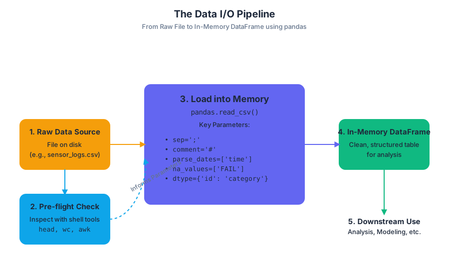
Before even attempting to load a large, unfamiliar file in Python, a prudent first step is to inspect it using command-line tools. This avoids memory errors and provides crucial metadata for crafting the correct read_csv call.
# Shell: Inspecting a CSV file before loading
# Assume the data is in a file named 'sensor_logs.csv'

# 1. View the first 5 lines to check the header and delimiter
$ head -n 5 sensor_logs.csv
# Sensor Log Data
# Collected on: 2023-10-27
# sensor_id;timestamp;reading_1;reading_2;status
# A-01;27/10/2023 08:00:15;10.5;88.1;OK
# B-02;27/10/2023 08:00:18;22.1;15.4;FAIL

# 2. Count the total number of lines to gauge file size
$ wc -l sensor_logs.csv
# 6 sensor_logs.csv

# 3. Use awk to check the number of fields in each line (using ';' as delimiter)
# This helps identify malformed rows. NF is the Number of Fields.
$ awk -F';' '{print NF}' sensor_logs.csv
# 1
# 1
# 5
# 5
# 5
# 5
This shell-level inspection reveals the semicolon delimiter, the two comment lines, and the consistent 5-column structure, informing the parameters we used in the Python code.
pd.read_csv Parameter |
Purpose | Common Use Case |
|---|---|---|
filepath_or_buffer |
The path to the file or a file-like object. | '/path/to/data.csv' or a URL. |
sep or delimiter |
The character sequence separating values. | ',' (default), '\t' for tab-separated, ';'. |
header |
Row number to use as column names. | 0 (default), None if no header. |
names |
A list of column names to use. | Used when header=None or to override existing headers. |
index_col |
Column to use as the row labels (index). | 0 to use the first column. |
dtype |
A dictionary mapping column names to data types. | {'user_id': str, 'value': float} to prevent incorrect type inference. |
parse_dates |
List of columns to parse as dates. | ['timestamp', 'event_date']. |
na_values |
Additional strings to recognize as NaN. |
['Not Available', 'N/A', -1]. |
chunksize |
An integer for iterating over a large file in chunks. | 100000 to process a multi-gigabyte file without loading it all into memory. |
Common Pitfalls
- Encoding Errors: Files saved with non-standard encoding (e.g.,
latin1) will raise aUnicodeDecodeErrorif not read with the correctencodingparameter. Always default toencoding='utf-8'if unsure. - Mixed Data Types: A column containing both numbers and text will be inferred as type
object, which is inefficient. This often triggers aDtypeWarning. Use thedtypeparameter to specify types explicitly or investigate the source of the mixed types. - Memory Overload: Attempting to load a file larger than available RAM will crash the session. For large files, use the
chunksizeparameter inread_csvto process the file piece by piece, or consider more scalable tools like Dask or Polars.
Subsetting & Filtering: The Art of Selection
What It Is
Subsetting is the process of extracting a portion of your data. This can involve selecting specific columns (projection), specific rows (selection), or a combination of both. Filtering is a form of subsetting rows based on one or more logical conditions. pandas provides a rich set of accessors for this purpose, primarily .loc, .iloc, and boolean indexing.
Definition: Accessors In
pandas, accessors like.locand.ilocare properties that provide a dedicated namespace for a specific type of indexing. They are not methods (called with()), but are used with square brackets[]. This design avoids ambiguity in the standard[]operator.
Why It Matters
Raw datasets are often vast and contain information irrelevant to the specific question at hand. Effective subsetting is the primary way to isolate the signal from the noise, focusing your computational resources and analytical attention on the relevant data. It is the pandas equivalent of the WHERE clause in SQL or filtering in a spreadsheet.
How It Works: Label vs. Position
pandas makes a critical distinction between label-based and position-based indexing.
.loc(Label-based): Selects data based on the index labels and column names. The slicing is inclusive of the endpoint.df.loc['start_label':'end_label']includes'end_label'..iloc(Integer-position-based): Selects data based on its integer position (from0tolength-1). The slicing follows Python's convention and is exclusive of the endpoint.df.iloc[0:5]includes positions 0, 1, 2, 3, and 4.- Boolean Indexing: A
SeriesofTrue/Falsevalues, with the same index as theDataFrame, can be passed to.locor the[]operator to select only the rows where the value isTrue.
Consider a dataset of employee records. We want to find all senior engineers in the R&D department hired after 2020. This requires a combination of column selection and conditional row filtering.
# Python: Complex filtering with .loc and boolean indexing
import pandas as pd
import numpy as np

# Create a sample DataFrame
data = {
    'employee_id': range(101, 111),
    'name': [f'Emp_{i}' for i in range(10)],
    'department': ['R&D', 'Sales', 'R&D', 'HR', 'R&D', 'Sales', 'R&D', 'HR', 'Sales', 'R&D'],
    'title': ['Engineer', 'Manager', 'Senior Engineer', 'Recruiter', 'Engineer', 'Analyst', 'Senior Engineer', 'Manager', 'Analyst', 'Data Scientist'],
    'hire_date': pd.to_datetime(['2019-03-15', '2018-07-22', '2021-01-10', '2022-05-30', '2023-08-01', '2019-11-12', '2022-02-14', '2021-09-01', '2023-04-18', '2020-12-01']),
    'salary': [75000, 110000, 120000, 65000, 82000, 70000, 135000, 105000, 72000, 150000]
}
employees = pd.DataFrame(data).set_index('employee_id')

# Define the conditions for filtering
is_rd = employees['department'] == 'R&D'
is_senior_engineer = employees['title'] == 'Senior Engineer'
hired_after_2020 = employees['hire_date'] > '2020-12-31'

# Combine conditions and apply the filter using .loc
# Select only the 'name', 'title', and 'salary' columns for the filtered rows
result = employees.loc[
    (is_rd & is_senior_engineer) & hired_after_2020,
    ['name', 'title', 'salary']
]

print(result)
This same logical query can be expressed elegantly in SQL, highlighting the conceptual parallels between database querying and DataFrame manipulation.
-- SQL: Equivalent filtering query
SELECT
    name,
    title,
    salary
FROM
    employees
WHERE
    department = 'R&D'
    AND title = 'Senior Engineer'
    AND hire_date > '2020-12-31';
| Feature | .loc |
.iloc |
|---|---|---|
| Selection By | Label | Integer Position |
| Arguments | Index/column labels | Integers, slices of integers |
| Slicing Endpoint | Inclusive (df.loc['a':'c'] includes 'c') |
Exclusive (df.iloc[0:3] includes 0, 1, 2) |
| Error Handling | KeyError if a label is not found |
IndexError if an integer is out of bounds |
| Use Case | When index/column names are meaningful and stable | When you need positional access, regardless of labels |
Common Pitfalls
- Chained Indexing and
SettingWithCopyWarning: A very common mistake is to use two sets of brackets to select and assign, likedf[df['col1'] > 0]['col2'] = 100. This is called chained indexing.pandascannot guarantee whether the first operation returns a view or a copy of the data, so the assignment might fail silently. This raises aSettingWithCopyWarning. - The Correct Approach: Always use
.locfor simultaneous row and column selection when assigning:df.loc[df['col1'] > 0, 'col2'] = 100. This is a single, unambiguous operation that always modifies the originalDataFrame.
Column Creation & Renaming: Shaping the Schema
What It Is
This involves two related operations:
- Column Creation: Adding new columns to a
DataFrame, typically derived from calculations on existing columns. This is the primary mechanism for feature engineering. - Column Renaming: Modifying the labels of columns (or the index) to be more descriptive, to conform to a standard, or to remove problematic characters.
Why It Matters
Raw data often lacks the explicit features needed for modeling or analysis. For example, a dataset might contain birth_date but not age, or revenue and cost but not profit. Creating these derived columns is a fundamental step in enriching the dataset. Renaming columns is a matter of good housekeeping, making the data easier to understand and work with, especially for collaborators.
How It Works: Vectorization and Chaining
The most efficient way to create new columns is through vectorized operations. Instead of looping through rows, you apply operations to entire Series at once. pandas, built on NumPy, is highly optimized for this.
There are two main syntactic styles for this:
- Direct Assignment: The classic
df['new_column'] = ...syntax. It's simple and modifies theDataFramein place. .assign()Method: A functional approach,df.assign(new_column=...). It does not modify the originalDataFramebut returns a new one with the added column. This makes it ideal for method chaining.
For renaming, the .rename() method is the standard tool. It accepts a dictionary mapping old names to new names.
# Python: Column creation and renaming
import pandas as pd
import numpy as np

# Sample sales data
sales_data = {
    'order_id': ['O1', 'O2', 'O3', 'O4'],
    'product_name': ['Widget A', 'Widget B', 'Widget A', 'Widget C'],
    'unit_price_usd': [10.00, 25.50, 10.25, 5.75],
    'quantity': [5, 2, 10, 8]
}
sales = pd.DataFrame(sales_data)

# --- Column Creation ---
# 1. Direct assignment (vectorized operation)
sales['total_price_usd'] = sales['unit_price_usd'] * sales['quantity']

# 2. Using .assign() for chaining, and a more complex function
# Let's add a 5% tax and convert to EUR (assume 1 USD = 0.92 EUR)
exchange_rate = 0.92
final_sales = (
    sales
    .assign(
        total_price_eur=lambda df: df['total_price_usd'] * 1.05 * exchange_rate,
        category=lambda df: df['product_name'].str.split().str[0]
    )
    # --- Renaming ---
    # Rename columns to a more standard format
    .rename(columns={
        'unit_price_usd': 'unit_price',
        'total_price_eur': 'final_price_eur',
        'quantity': 'units_sold'
    })
)

print("Original DataFrame:")
print(sales)
print("\nTransformed DataFrame:")
print(final_sales)
The same transformations can be achieved in R using the popular dplyr library, which heavily emphasizes a chainable, "pipe-based" workflow that is conceptually similar to pandas's method chaining.
# R/dplyr: Equivalent data manipulation
library(dplyr)

# Create the initial data frame
sales_data <- data.frame(
  order_id = c('O1', 'O2', 'O3', 'O4'),
  product_name = c('Widget A', 'Widget B', 'Widget A', 'Widget C'),
  unit_price_usd = c(10.00, 25.50, 10.25, 5.75),
  quantity = c(5, 2, 10, 8)
)

exchange_rate <- 0.92

# Use pipes (%>%) to chain operations
final_sales <- sales_data %>%
  # Create new columns with mutate()
  mutate(
    total_price_usd = unit_price_usd * quantity,
    final_price_eur = total_price_usd * 1.05 * exchange_rate,
    category = sapply(strsplit(product_name, " "), `[`, 1)
  ) %>%
  # Rename columns with rename()
  rename(
    unit_price = unit_price_usd,
    units_sold = quantity
  )

print(final_sales)
Grouping & Aggregation: Summarizing with Precision
What It Is
Grouping and Aggregation is a powerful process for computing summary statistics on subsets of data. It is famously described by the "split-apply-combine" paradigm:
- Split: The data is partitioned into groups based on the values in one or more key columns.
- Apply: A function (the aggregation) is applied independently to each group. This could be a sum, mean, count, or a custom function.
- Combine: The results of the function applications are combined into a new
DataFrame.
The cornerstone of this process in pandas is the .groupby() method.
AI_DEMOI_DEMO### Why It Matters Raw, row-level data is often too granular to reveal meaningful patterns. Aggregation allows you to zoom out and see the bigger picture. How do sales compare across different regions? What is the average patient recovery time for different treatment groups? What is the maximum error rate per sensor type? These are all questions that can only be answered through grouping and aggregation. It is the engine of descriptive analytics.
How It Works: The GroupBy Object
Calling df.groupby('key_column') does not immediately compute anything. Instead, it returns a DataFrameGroupBy object. This is a lazy object that holds all the information needed to perform computations on the groups. The actual calculation happens only when an aggregation method (like .sum(), .mean(), .size(), or .agg()) is called on this object.
The .agg() method is the most flexible, allowing you to apply multiple functions at once, and even apply different functions to different columns.
# Python: Advanced aggregation with .groupby().agg()
import pandas as pd

# Sample dataset of customer transactions
data = {
    'customer_id': ['C1', 'C2', 'C1', 'C3', 'C2', 'C1'],
    'region': ['North', 'South', 'North', 'North', 'West', 'West'],
    'product_category': ['Electronics', 'Apparel', 'Home Goods', 'Electronics', 'Apparel', 'Electronics'],
    'sales': [1200, 150, 450, 800, 200, 1500],
    'quantity': [1, 3, 2, 1, 4, 2]
}
transactions = pd.DataFrame(data)

# Group by region and customer, then compute multiple aggregations
# We want total sales, average sale amount, and number of unique product categories per group
summary = transactions.groupby(['region', 'customer_id']).agg(
    total_sales=('sales', 'sum'),
    average_sale=('sales', 'mean'),
    distinct_categories=('product_category', 'nunique'),
    number_of_transactions=('sales', 'count')
)

print(summary)
This split-apply-combine pattern is a direct analogue to SQL's GROUP BY clause, which is the canonical implementation of this idea in the database world.
-- SQL: Equivalent GROUP BY query
SELECT
    region,
    customer_id,
    SUM(sales) AS total_sales,
    AVG(sales) AS average_sale,
    COUNT(DISTINCT product_category) AS distinct_categories,
    COUNT(sales) AS number_of_transactions
FROM
    transactions
GROUP BY
    region,
    customer_id
ORDER BY
    region,
    customer_id;
Variations: transform and filter
While agg returns a reduced summary, groupby has other powerful methods:
.transform(func): Applies a function to each group but returns aSeriesorDataFramewith the same index as the original. This is useful for creating group-level features, like a column showing the average sales for each customer's region on every transaction row..filter(func): Takes a function that returnsTrueorFalsefor each group. It then returns a subset of the originalDataFramecontaining only the rows from groups where the function returnedTrue. This is useful for discarding groups that don't meet a certain criterion (e.g., keeping only customers with more than 2 transactions).
GroupBy Method |
Output Shape | Common Use Case |
|---|---|---|
agg() |
Reduced; one row per group. | Calculating summary statistics (sum, mean, count). |
transform() |
Same as input. | Creating new columns based on group properties (e.g., z-scores within a group). |
filter() |
Subset of input rows. | Dropping entire groups based on a condition (e.g., groups with too few members). |
Combining & Merging Data: Assembling the Puzzle
What It Is
Combining is the process of integrating data from two or more DataFrames into a single one. pandas provides two primary mechanisms for this:
pd.concat(): StacksDataFrameson top of each other (row-wise,axis=0) or side-by-side (column-wise,axis=1). It aligns data based on the index.pd.merge(): Performs database-style joins onDataFrames. It combines them based on the values in one or more common columns (the "keys").
Why It Matters
In any real-world project, data is fragmented. Customer information might be in one table, their orders in another, and product details in a third. To get a complete picture—for instance, to find the total sales for customers in a specific demographic—you must combine these disparate datasets. Merging is the core operation for linking related data.
How It Works: Concatenation vs. Merging
Concatenation is like gluing pieces of paper together. It's a simple, positional operation. When concatenating by rows, pandas appends the rows and aligns the columns. If a column exists in one DataFrame but not another, it will be filled with NaN in the respective rows.
Merging, on the other hand, is a more sophisticated, value-based operation rooted in relational algebra. It combines rows from two DataFrames where the values in their key columns match. The type of join determines how to handle keys that don't exist in both DataFrames.
Definition: Join Types
- Inner Join: Returns only the rows where the key exists in both
DataFrames. This is the intersection of the keys.- Left Join: Returns all rows from the left
DataFrame, and the matched rows from the rightDataFrame. If there is no match for a key from the leftDataFrame, the columns from the right will beNaN.- Right Join: The reverse of a left join. Returns all rows from the right
DataFrame.- Outer Join: Returns all rows when there is a match in either the left or the right
DataFrame. This is the union of the keys.
Let's say we have one DataFrame with employee details and another with their department information. We can use a merge to add the department name and location to each employee's record.
# Python: A realistic pd.merge() example
import pandas as pd

employees = pd.DataFrame({
    'emp_id': ['E1', 'E2', 'E3', 'E4', 'E5'],
    'name': ['Alice', 'Bob', 'Charlie', 'David', 'Eve'],
    'dept_code': ['D1', 'D2', 'D1', 'D3', 'D2']
})

departments = pd.DataFrame({
    'department_id': ['D1', 'D2', 'D4'],
    'department_name': ['Engineering', 'Marketing', 'Legal'],
    'location': ['Building A', 'Building B', 'Building C']
})

# Perform a left merge to keep all employees, even if their department is missing
# Note the use of `left_on` and `right_on` because the key columns have different names
employee_full_details = pd.merge(
    left=employees,
    right=departments,
    how='left',
    left_on='dept_code',
    right_on='department_id'
)

print(employee_full_details)
The result will show all five employees. David (dept D3) and any employee in a department not listed in the departments DataFrame will have NaN for department_name and location. The Legal department (D4) will not appear at all because no employee belongs to it.
The logic of these joins can be formally expressed using set theory, where A and B are the sets of keys in the left and right tables, respectively.
# Mathematical: Set theory representation of joins

Inner Join Keys = A ∩ B
Left Join Keys  = A
Right Join Keys = B
Outer Join Keys = A ∪ B
merge Parameter |
Purpose | Example |
|---|---|---|
left, right |
The two DataFrames to merge. |
pd.merge(df1, df2, ...) |
how |
The type of join to perform. | 'inner', 'left', 'right', 'outer' |
on |
Column name(s) to join on. Must be present in both DataFrames. |
on='customer_id' |
left_on, right_on |
Column names to join on when key names differ. | left_on='user_key', right_on='id' |
suffixes |
A tuple of strings to append to overlapping column names (not keys). | ('_left', '_right') |
indicator |
If True, adds a column _merge indicating the source of each row. |
True |
Reshaping Data: Changing Perspective
What It Is
Reshaping refers to changing the layout of a DataFrame's data, often to make it "wider" or "longer." This is done without altering the actual data values, only their organization. The two primary reshaping operations are:
- Pivoting: Transforms data from a "long" format to a "wide" format. It takes unique values from one column and makes them into new columns.
- Melting: The inverse of pivoting. It transforms data from a "wide" format to a "long" format, turning columns into rows.
These operations are guided by the principles of Tidy Data, where each variable forms a column, each observation forms a row, and each type of observational unit forms a table.
Why It Matters
The "shape" of your data can dramatically affect how easy it is to analyze or visualize. Most statistical modeling and plotting libraries (like statsmodels and seaborn) expect data in a "long," tidy format. However, data is often recorded or presented in a "wide" format that is more human-readable (like a spreadsheet). Being able to seamlessly transition between these formats is a critical skill.
How It Works: pivot and melt
pivot_table(): Creates a spreadsheet-style pivot table. You specify which column should become the newindex, which column's values should become the newcolumns, and which column should provide thevaluesto fill the table. It's more robust than the basic.pivot()because it can aggregate values if there are duplicate entries for a given index/column pair..melt(): "Unpivots" aDataFrame. You specify which columns areid_vars(identifier variables that should remain as columns) and the rest of the columns are consideredvalue_vars, which are unpivoted into two new columns: one for the variable name and one for the value.
Let's see this in action. We start with wide-format quarterly sales data and transform it into a long, tidy format, which is better for plotting time series.
# Python: Reshaping with melt and pivot_table
import pandas as pd

# Wide-format data: easy for humans to read
wide_data = pd.DataFrame({
    'country': ['USA', 'Germany', 'USA', 'Germany'],
    'product': ['A', 'A', 'B', 'B'],
    'Q1_2023': [100, 80, 50, 40],
    'Q2_2023': [110, 85, 60, 42],
    'Q3_2023': [120, 90, 55, 45]
})

# --- Melt: From Wide to Long ---
# This format is ideal for analysis and plotting
long_data = wide_data.melt(
    id_vars=['country', 'product'],
    var_name='quarter',
    value_name='sales'
)

# --- Pivot: From Long back to Wide ---
# Let's pivot to see total sales per country for each quarter
# The aggregation function (aggfunc) is needed because there are multiple products per country
pivoted_data = long_data.pivot_table(
    index='country',
    columns='quarter',
    values='sales',
    aggfunc='sum' # Aggregate the sales for products A and B
)

print("--- Original Wide Data ---")
print(wide_data)
print("\n--- Melted (Long) Data ---")
print(long_data)
print("\n--- Pivoted Back (Aggregated Wide) Data ---")
print(pivoted_data)
This same wide-to-long transformation is a core concept in R's tidyr package, part of the Tidyverse. The functions pivot_longer() and pivot_wider() are the direct equivalents of melt and pivot_table.
# R/tidyr: Equivalent reshaping operations
library(tidyr)
library(dplyr)

# Create the wide data frame
wide_data <- data.frame(
  country = c('USA', 'Germany', 'USA', 'Germany'),
  product = c('A', 'A', 'B', 'B'),
  Q1_2023 = c(100, 80, 50, 40),
  Q2_2023 = c(110, 85, 60, 42),
  Q3_2023 = c(120, 90, 55, 45)
)

# --- pivot_longer: From Wide to Long ---
long_data <- wide_data %>%
  pivot_longer(
    cols = starts_with("Q"),
    names_to = "quarter",
    values_to = "sales"
  )

# --- pivot_wider: From Long to Wide ---
pivoted_data <- long_data %>%
  group_by(country, quarter) %>%
  summarise(total_sales = sum(sales)) %>%
  pivot_wider(
    names_from = quarter,
    values_from = total_sales
  )

print("--- Melted (Long) Data in R ---")
print(long_data)
print("--- Pivoted Back (Wide) Data in R ---")
print(pivoted_data)
Common Pitfalls
- Pivoting with Duplicate Entries: Using
.pivot()will raise an error if you have duplicate values for the chosenindexandcolumns. For example, if thewide_dataabove had two rows forUSAand productA. This is the primary reason to preferpivot_table(), as it forces you to choose an aggregation function (aggfunc) to handle these duplicates explicitly. - Choosing
id_varsinmelt: Forgetting to include a column inid_varsmeans it will be melted down into the variable/value columns, which is usually not the desired outcome. Always double-check that all identifier columns are correctly specified.
Source Materials
Study pandas documentation on Lykke
This course page is free to open: signed out, you can read its first two sections, and signing in, on any plan, opens the rest. The free Lykke Chrome extension syncs your own Canvas courses, so ChatGPT, Claude and Muse can answer from your classes and deadlines. It only reads Canvas.
Add the free extensionSign in to open every sectionAll sections of pandas documentation · Browse more course pages