From the free course pandas documentation on Lykke
Advanced Data Handling: Time Series and Text
Key concepts: Time Series Conversion (pd.to_datetime) · Datetime Properties (.dt accessor) · DatetimeIndex and Slicing · Time Frequency Resampling (.resample) · Vectorized String Operations (.str accessor) · String Splitting and Filtering
This section dives into specialized techniques for handling two common but complex data types: time series and text. You will learn how to leverage pandas' built-in functionalities to parse dates, perform time-based analysis, and manipulate string data efficiently.
Advanced Data Handling: Time Series and Text
Beyond the clean, numerical data often found in textbooks, real-world datasets are frequently populated with temporal and textual information. Financial transactions are timestamped, server logs record events in sequence, and user feedback arrives as unstructured text. To perform meaningful analysis, we must first tame these complex data types. The pandas library provides a sophisticated, high-performance toolkit for this purpose, centered around two powerful constructs: the datetime object for time series and the vectorized string accessor for text. This section provides a deep dive into the principles and practices of manipulating these essential data formats.
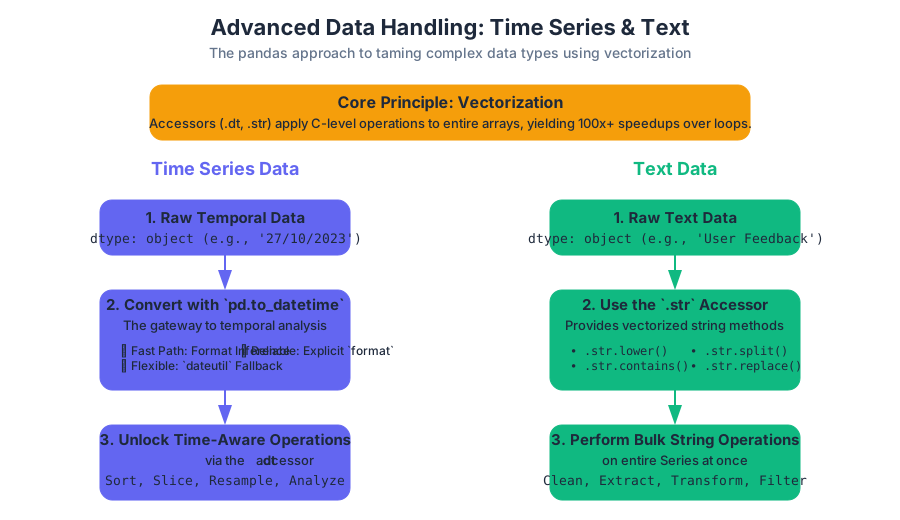
AI_SVGI_SVG Core Principle: Vectorization
The central theme connecting the handling of both time series and text data in pandas is vectorization. Instead of writing slow, explicit
forloops in Python, we use specialized accessors (.dtand.str) that apply operations to entire arrays of data at the C level. This approach is not merely a convenience; it is a fundamental performance paradigm that can yield speedups of 100x or more, making it possible to process millions of records in seconds.
Time Series Conversion: The Gateway to Temporal Analysis
The journey into time series analysis begins with a crucial first step: converting raw, ambiguous representations of dates and times into a structured, machine-readable format. This is the role of pd.to_datetime.
What it is: pd.to_datetime
pd.to_datetime is a highly optimized and flexible function that parses a wide variety of string, integer, or float representations and converts them into pandas Timestamp objects. A Timestamp is the pandas equivalent of Python's datetime.datetime object but is built upon the more efficient numpy.datetime64[ns] data type, providing nanosecond precision and enabling storage in contiguous memory blocks.
The function is the cornerstone of all time series functionality. Without this explicit conversion, a column of date strings like "2023-10-27" is treated as generic text, sorting lexicographically (e.g., "01-12-2024" would come before "27-10-2023") and prohibiting any form of temporal arithmetic.
Why it matters: Unlocking Time-Aware Operations
Converting data to a datetime format is not just about data typing; it's about unlocking a vast ecosystem of time-aware capabilities. Once converted, data can be:
- Sorted Chronologically: The most fundamental requirement for time series analysis.
- Sliced and Indexed by Date: Selecting data for "October 2023" becomes a trivial operation.
- Used in Temporal Arithmetic: Calculating durations between events (e.g.,
time_to_purchase = purchase_ts - view_ts). - Resampled to Different Frequencies: Aggregating daily data into monthly summaries or vice-versa.
- Analyzed for Seasonality and Trends: Decomposing the timestamp into components like "day of the week" or "quarter of the year".
How it works: Parsing and Inference
Internally, pd.to_datetime employs a multi-layered parsing strategy for both flexibility and speed.
- Format Inference: For array-like inputs, pandas first attempts to infer a common date format. If it finds one (e.g., all strings are in
YYYY-MM-DDformat), it uses a highly optimized, vectorized internal routine to perform the conversion. This is the fastest path. dateutil.parserFallback: If inference fails due to inconsistent or complex formats, pandas falls back to thedateutil.parser.parsefunction for each individual element. This parser is incredibly flexible and can understand formats like"October 27th, 2023", but it is significantly slower as it operates on an element-by-element basis.- Explicit Formatting: The user can provide an explicit format string via the
formatargument (e.g.,format='%d-%m-%Y'). This bypasses inference and thedateutilfallback, guaranteeing the fastest and most reliable parsing path, provided the data is clean.
Concrete Example: From Raw Logs to Datetime Objects
Imagine we have a log file from a web server with timestamps in various, slightly inconsistent formats. Our goal is to parse these into a usable datetime column.
import pandas as pd
import numpy as np

# Raw data with inconsistent formats and an invalid entry
log_data = [
    '2023-10-27 08:30:15',
    '28/10/2023 09:12:05',
    'Oct 29, 2023 11:00:00',
    'Invalid Timestamp',
    '2023-10-30 14:22:30'
]
df = pd.DataFrame(log_data, columns=['raw_timestamp'])

# Convert using pd.to_datetime, coercing errors to NaT (Not a Time)
df['timestamp'] = pd.to_datetime(df['raw_timestamp'], errors='coerce')

# Display the result, showing the parsed datetimes and the NaT
print("--- Parsed Timestamps ---")
print(df)
print("\n--- Data Types ---")
print(df.dtypes)
Output:
--- Parsed Timestamps ---
           raw_timestamp           timestamp
0  2023-10-27 08:30:15 2023-10-27 08:30:15
1  28/10/2023 09:12:05 2023-10-28 09:12:05
2  Oct 29, 2023 11:00:00 2023-10-29 11:00:00
3      Invalid Timestamp                 NaT
4  2023-10-30 14:22:30 2023-10-30 14:22:30

--- Data Types ---
raw_timestamp            object
timestamp        datetime64[ns]
dtype: object
Notice how pd.to_datetime correctly interpreted three different formats and gracefully handled the invalid string by converting it to NaT when errors='coerce' was specified.
In a production pipeline, you might pre-process these logs at the command line before they even enter a Python environment.
# Using awk to attempt to reformat a log file into a consistent ISO 8601 format
# This is a simplified example; a real-world script would be more robust.
# cat server.log | awk '{ ... complex reformatting logic ... }' > cleaned_server.log

# Example: Reformat a DD/MM/YYYY date to YYYY-MM-DD using sed
echo "28/10/2023 09:12:05" | sed -E 's|([0-9]{2})/([0-9]{2})/([0-9]{4})|\3-\2-\1|'
# Output: 2023-10-28 09:12:05
This demonstrates that data cleaning is a multi-stage process, and standardizing formats early can simplify downstream processing in pandas.
Variations / Extensions: Parameterization
The pd.to_datetime function is highly configurable. The table below summarizes its most critical parameters.
| Parameter | Type | Description | Common Use Case |
|---|---|---|---|
arg |
Series, list, str |
The data to be converted. | The primary input data. |
errors |
str |
How to handle parsing errors. 'raise' (default), 'coerce' (set to NaT), 'ignore' (return original input). |
Use 'coerce' for dirty data to avoid script failure. |
format |
str |
The specific strftime format string. |
Massively improves performance on clean, consistent data. |
dayfirst |
bool |
Whether to interpret ambiguous dates like 10/11/12 as DD/MM/YY (True) or MM/DD/YY (False, default). |
Essential when working with European date formats. |
yearfirst |
bool |
Whether to interpret ambiguous dates like 10/11/12 as YY/MM/DD. |
Less common, but useful for certain international formats. |
utc |
bool |
If True, returns a timezone-aware UTC DatetimeIndex. |
Standardizing timestamps from different sources to a single timezone. |
Common Pitfalls
- Timezone Naivety: By default,
pd.to_datetimeproduces timezone-naivedatetimeobjects. This can lead to serious errors when combining data from different geographic locations. Always consider usingtz_localizeto assign a timezone to naive timestamps ortz_convertto switch between timezones. - Performance on Mixed Formats: Relying on the
dateutilfallback for millions of rows with inconsistent formats will be a major performance bottleneck. The best practice is to clean and standardize date strings as much as possible before callingpd.to_datetime, and then use theformatargument.
The Datetime Accessor: Decomposing Time
Once a Series is of datetime64 type, you gain access to the .dt accessor. This powerful tool is the key to feature engineering from temporal data.
What it is: The .dt Accessor
The .dt accessor is a special property available on pandas Series that contain datetime-like values. It exposes a wide range of properties and methods for extracting temporal components in a vectorized manner. For example, series.dt.year returns a new Series containing the year of each timestamp.
Why it matters: Feature Engineering from Time
A raw timestamp like 2023-10-27 08:30:15.123456789 is a high-cardinality feature that is nearly useless to most machine learning models. Its value is in its components. By decomposing it, we can create meaningful features that capture patterns and seasonality:
- Is there a difference in user activity on weekends vs. weekdays? (
.dt.weekdayor.dt.day_name()) - Do sales peak in the last month of the quarter? (
.dt.month,.dt.quarter) - Is there a specific hour of the day when server load is highest? (
.dt.hour)
The .dt accessor makes creating these features trivial and computationally efficient.
Concrete Example: Analyzing User Login Patterns
Let's analyze a dataset of user login timestamps to identify the busiest days of the week and hours of the day.
# Generate a realistic series of 10,000 login timestamps over a month
rng = np.random.default_rng(0)
base_time = pd.to_datetime('2023-10-01')
random_seconds = rng.integers(0, 30*24*3600, size=10000)
login_timestamps = base_time + pd.to_timedelta(random_seconds, unit='s')
logins = pd.Series(login_timestamps, name='login_time').sort_values()

# --- Feature Engineering with .dt accessor ---
df = pd.DataFrame(logins)
df['day_of_week'] = df['login_time'].dt.day_name()
df['hour_of_day'] = df['login_time'].dt.hour

# --- Analysis ---
# Find the busiest hour of the day
busiest_hour = df['hour_of_day'].value_counts().nlargest(1)
print(f"Busiest hour of the day:\n{busiest_hour}\n")

# Find the busiest day of the week
day_order = ["Monday", "Tuesday", "Wednesday", "Thursday", "Friday", "Saturday", "Sunday"]
busiest_day = df['day_of_week'].value_counts().loc[day_order]
print(f"Logins by day of the week:\n{busiest_day}")
Output:
Busiest hour of the day:
hour_of_day
18    453
Name: count, dtype: int64

Logins by day of the week:
day_of_week
Monday       1403
Tuesday      1429
Wednesday    1433
Thursday     1407
Friday       1469
Saturday     1447
Sunday       1412
Name: count, dtype: int64
This example shows a complete mini-analysis: we took raw timestamps, used .dt to engineer meaningful categorical features, and then used standard pandas methods like .value_counts() to derive insights.
Variations / Extensions: The Breadth of .dt Properties
The .dt accessor provides a rich set of attributes.
| Property/Method | Returns | Description |
|---|---|---|
.year, .month, .day |
int |
The corresponding integer value for the date component. |
.hour, .minute, .second |
int |
The corresponding integer value for the time component. |
.weekday |
int |
The day of the week, where Monday=0 and Sunday=6. |
.day_name() |
str |
The full name of the day (e.g., "Monday"). |
.month_name() |
str |
The full name of the month (e.g., "October"). |
.quarter |
int |
The quarter of the year (1-4). |
.is_month_start |
bool |
True if the date is the first day of the month. |
.is_year_end |
bool |
True if the date is the last day of the year. |
.strftime('%Y-%m-%d') |
str |
Formats the datetime back into a string with a custom format. |
.round('H') |
datetime |
Rounds the timestamp to the nearest specified frequency (e.g., hour). |
The DatetimeIndex: Supercharging Selection and Slicing
While the .dt accessor operates on Series, the true power of pandas time series is realized when a datetime column is set as the DataFrame's index, creating a DatetimeIndex.
What it is: A Time-Based Index
A DatetimeIndex is a specialized pandas Index object composed of Timestamp objects. It is optimized for time-based data access and alignment. You can create one by passing a datetime Series to df.set_index().
Why it matters: Intuitive and Efficient Time-Based Queries
A DatetimeIndex revolutionizes how you select data. Instead of complex boolean filtering like df[(df['date'] >= '2023-10-01') & (df['date'] < '2023-11-01')], you can use concise, intuitive string-based slicing.
Key Insight:
DatetimeIndexenables label-based slicing with partial date strings.df['2023']selects all data for the year 2023.df['2023-10']selects all data for October 2023. This is not just syntactic sugar; it's a gateway to high-performance time-window queries.
How it works: Under the Hood
The performance of DatetimeIndex comes from its underlying structure. It is backed by a monotonic numpy.datetime64[ns] array. When you perform a slice like df['2023-10-01':'2023-10-15'], pandas doesn't need to scan every row. Because the index is sorted, it can use efficient search algorithms (like binary search) to quickly locate the start and end positions of the slice, making lookups extremely fast, often O(log N).
Concrete Example: Slicing Financial Stock Data
Consider a DataFrame of daily stock prices indexed by date.
# Create a sample DataFrame with a DatetimeIndex
dates = pd.date_range(start='2023-01-01', end='2023-12-31', freq='D')
data = {
    'price': 100 + np.random.randn(len(dates)).cumsum(),
    'volume': np.random.randint(1_000_000, 5_000_000, size=len(dates))
}
stocks_df = pd.DataFrame(data, index=dates)
stocks_df.index.name = 'date'

print("--- Original DataFrame Head ---")
print(stocks_df.head())

# --- Slicing Examples ---

# 1. Select a single day's data
print("\n--- Data for October 27, 2023 ---")
print(stocks_df.loc['2023-10-27'])

# 2. Select an entire month (October 2023)
print("\n--- Data for October 2023 ---")
october_data = stocks_df['2023-10']
print(october_data.head(2))
print(october_data.tail(2))

# 3. Select a specific date range (first two weeks of Q4)
print("\n--- Data for Q4 Start (Oct 1 to Oct 14, 2023) ---")
q4_start = stocks_df.loc['2023-10-01':'2023-10-14']
print(q4_start)
AI_DEMOI_DEMOhis code demonstrates the elegance and power of DatetimeIndex slicing. The syntax is clean, readable, and internally optimized for performance.
Time Frequency Resampling: Aggregating and Interpolating
Resampling is the process of converting a time series from one frequency to another. It is a fundamental operation for summarizing data, aligning disparate datasets, and filling in missing values.
What it is: The .resample() Method
The .resample() method is a time-based groupby operation. It is called on a Series or DataFrame with a DatetimeIndex and is immediately followed by an aggregation (.sum(), .mean(), .ohlc()) or interpolation (.asfreq(), .ffill()) method.
There are two primary types of resampling:
- Downsampling: Aggregating data from a high frequency to a low frequency (e.g., daily data to monthly data). This reduces the number of rows and requires an aggregation function to combine the data points within each new period (e.g.,
sum()of daily sales to get monthly sales). - Upsampling: Converting data from a low frequency to a high frequency (e.g., daily data to hourly data). This increases the number of rows and introduces missing values, which must be filled using a method like forward-fill (
.ffill()) or interpolation (.interpolate()).
Why it matters: Aligning and Summarizing Data
Resampling is critical for:
- Creating Reports: Generating quarterly or annual summaries from daily operational data.
- Noise Reduction: Smoothing out volatile, high-frequency data to reveal underlying trends.
- Data Alignment: Aligning two datasets with different frequencies (e.g., daily sales and weekly marketing spend) before modeling their relationship.
How it works: The Split-Apply-Combine Paradigm
The .resample() method follows the classic "split-apply-combine" pattern:
- Split: The
DatetimeIndexis conceptually divided into time bins according to the target frequency (e.g., for.resample('M'), all data points from October 1st to October 31st fall into the "October" bin). - Apply: An aggregation function is applied to the data within each bin. For example,
.mean()calculates the average of all values in that bin. - Combine: The results of the aggregation for each bin are collected into a new Series or DataFrame, indexed by the end (or start) of each time bin.
Concrete Example: From Daily Sales to Monthly Totals
Let's downsample a daily sales dataset to get a monthly summary.
# Using the stocks_df from the previous example, let's treat 'volume' as 'daily_sales'
sales_df = stocks_df[['volume']].rename(columns={'volume': 'daily_sales'})

# Resample daily sales to monthly totals
# 'M' stands for month-end frequency
monthly_sales = sales_df.resample('M').sum()
print("--- Monthly Sales Totals (Sum) ---")
print(monthly_sales)

# Resample to quarterly averages
# 'Q' stands for quarter-end frequency
quarterly_avg_sales = sales_df.resample('Q').mean()
print("\n--- Quarterly Average Daily Sales ---")
print(quarterly_avg_sales)
Output:
--- Monthly Sales Totals (Sum) ---
            daily_sales
date
2023-01-31     93333939
2023-02-28     83196887
2023-03-31     93175891
...
2023-12-31     92900983

--- Quarterly Average Daily Sales ---
                 daily_sales
date
2023-03-31      3.000064e+06
2023-06-30      2.990425e+06
2023-09-30      3.007687e+06
2023-12-31      3.021021e+06
This is a standard operation in business intelligence. The equivalent operation in SQL would use a date truncation function.
-- SQL equivalent for calculating monthly total sales
SELECT
  DATE_TRUNC('month', sale_date) AS month,
  SUM(sales_amount) AS total_sales
FROM
  sales
GROUP BY
  DATE_TRUNC('month', sale_date)
ORDER BY
  month;
This comparison highlights how .resample() provides a concise, powerful syntax for a common and critical database operation.
Vectorized String Operations: The .str Accessor
Just as the .dt accessor unlocks temporal data, the .str accessor is the key to processing textual data efficiently.
What it is: The .str Accessor
The .str accessor is a property on pandas Series with object dtype (typically containing strings) that exposes vectorized versions of Python's standard string methods. This allows you to apply string manipulations to an entire Series at once, without writing an explicit Python loop.
Why it matters: Avoiding Slow Python Loops
The performance difference between a vectorized .str operation and a Python loop is staggering.
# Performance comparison: Vectorized vs. Loop
import timeit

s = pd.Series(['string ' * 5] * 10000)

# Vectorized approach
vector_time = timeit.timeit(lambda: s.str.upper().str.strip(), number=100)

# Loop-based approach (using .apply with a lambda)
loop_time = timeit.timeit(lambda: s.apply(lambda x: x.upper().strip()), number=100)

print(f"Vectorized (.str) time: {vector_time:.4f} seconds")
print(f"Loop (.apply) time:     {loop_time:.4f} seconds")
print(f"Speedup: {loop_time / vector_time:.1f}x")

# On a typical machine, this will show a 10-50x speedup for the vectorized version.
This is because .str methods operate on the data at a lower level (often in C), avoiding the significant overhead of the Python interpreter for each element in the Series.
Concrete Example: Cleaning User-Entered Data
A common task is cleaning inconsistent text fields, such as product names entered by users.
# Messy product names
products = pd.Series([
    '  Product A ', 'product b', ' PRODUCT C', np.nan, 'Product_D'
])

# Chained .str methods for cleaning
cleaned_products = (
    products
    .str.strip()          # Remove leading/trailing whitespace
    .str.lower()          # Convert to lowercase
    .str.replace('_', ' ') # Replace underscores with spaces
)

print("--- Before Cleaning ---")
print(products)
print("\n--- After Cleaning ---")
print(cleaned_products)
Output:
--- Before Cleaning ---
0      Product A
1        product b
2       PRODUCT C
3             NaN
4       Product_D
dtype: object

--- After Cleaning ---
0    product a
1    product b
2    product c
3          NaN
4    product d
dtype: object
Note how NaN values are gracefully propagated through the chain of operations, which is the desired behavior in most data cleaning pipelines.
String Splitting and Filtering
Beyond simple cleaning, the .str accessor provides powerful methods for splitting strings into multiple columns and filtering rows based on complex patterns, often using regular expressions.
What it is: Pattern Matching and Extraction
This category includes methods like:
.str.contains(pat): Returns a booleanSeriesindicating if the patternpatis found in each string..str.split(pat, expand=True): Splits each string by the patternpatand expands the results into a new DataFrame..str.extract(pat): Uses a regular expression with capturing groups to extract substrings into new columns in a DataFrame.
Why it matters: Structuring Unstructured Text
These methods are the workhorses for converting semi-structured text into a fully structured, tabular format. A log entry like "ERROR:DB-01:Connection timed out" is not easily analyzable until it is split into Level, Source, and Message columns.
How it works: Regular Expressions as a First-Class Citizen
The true power of these methods is unlocked by regular expressions (regex). By setting regex=True (the default for many methods), you can define sophisticated patterns for matching and extraction.
.str.contains()becomes a powerful filter for finding records that match a complex rule..str.split(expand=True)is the fastest way to break apart delimited data..str.extract()is surgical. It uses parentheses()in the regex pattern to define capturing groups. Each group becomes a new column in the output DataFrame, containing only the text that matched that part of the pattern.
Concrete Example: Parsing Server Log Entries
Let's parse a Series of log entries to filter for errors and extract structured information.
logs = pd.Series([
    'INFO:2023-10-27:192.168.1.1:User logged in successfully',
    'WARN:2023-10-27:192.168.1.1:Login attempt failed',
    'ERROR:2023-10-28:10.0.0.5:Database connection failed: timeout',
    'INFO:2023-10-28:192.168.1.2:File uploaded'
])
df = pd.DataFrame({'log_entry': logs})

# 1. Filter for only ERROR messages
error_logs = df[df['log_entry'].str.contains('^ERROR')]
print("--- Error Logs Only ---")
print(error_logs)

# 2. Split the log entry into structured columns
# We use .str.split with a limit (n=3) to avoid splitting the message itself
log_parts = df['log_entry'].str.split(':', n=3, expand=True)
log_parts.columns = ['level', 'date', 'ip_address', 'message']
print("\n--- Parsed Log DataFrame ---")
print(log_parts)
Output:
--- Error Logs Only ---
                                           log_entry
2  ERROR:2023-10-28:10.0.0.5:Database connection ...

--- Parsed Log DataFrame ---
   level        date  ip_address                       message
0   INFO  2023-10-27  192.168.1.1  User logged in successfully
1   WARN  2023-10-27  192.168.1.1         Login attempt failed
2  ERROR  2023-10-28    10.0.0.5   Database connection failed: timeout
3   INFO  2023-10-28  192.168.1.2                 File uploaded
For more complex extraction, like pulling a username and action from a message, .str.extract() is superior. Consider a regex for a different log format.
# A regex to parse an Apache common log format entry
# It has capturing groups for IP, timestamp, request, status, and size.
^(\S+) \S+ \S+ \[(.*?)\] "(\S+ \S+ \S+)" (\d{3}) (\d+)$
Using this pattern with .str.extract() on Apache logs would instantly produce a structured DataFrame with five columns, a task that would be incredibly tedious and slow using manual string processing.
Common Pitfalls
- Greedy Regex: A common regex mistake is a "greedy" pattern like
.*that matches more than intended. Use non-greedy.*?or more specific character classes. - Performance of Complex Regex: While much faster than Python loops, a poorly written, inefficient regex can still be slow on very large datasets. Test and profile your patterns.
- Forgetting
expand=True: A call to.str.split()withoutexpand=Truereturns aSeriesof lists, which is often less useful than the DataFrame produced when it is set toTrue.
Source Materials
Study pandas documentation on Lykke
This course page is free to open: signed out, you can read its first two sections, and signing in, on any plan, opens the rest. The free Lykke Chrome extension syncs your own Canvas courses, so ChatGPT, Claude and Muse can answer from your classes and deadlines. It only reads Canvas.
Add the free extensionSign in to open every sectionAll sections of pandas documentation · Browse more course pages