From the free course Numerical Analysis and Computational Methods on Lykke
Root-Finding for Nonlinear Equations
Key concepts: Bisection Method · Newton's Method · Secant Method · Convergence Rates
Methods for finding the zeros of functions where analytical solutions are unavailable.
Root-Finding for Nonlinear Equations
Root-finding is one of the most fundamental challenges in numerical analysis. At its core, the problem is deceptively simple: given a continuous function $f(x)$, find the values of $x$ (roots or zeros) such that $f(x) = 0$. While linear equations can be solved using basic algebra, nonlinear equations—ranging from simple polynomials like $x^2 - 5 = 0$ to transcendental equations involving logarithms and trigonometry like $e^{-x} - \sin(x) = 0$—often lack analytical solutions.
In engineering and scientific computing, root-finding is the "engine" behind optimization, equilibrium analysis, and inverse modeling. Whether calculating the interest rate of a complex loan, determining the depth of a floating buoy, or finding the steady-state temperature of a heat sink, we are almost always solving for a root.
The Mathematical Foundation: Bracketing vs. Open Methods
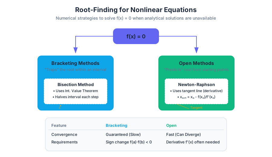
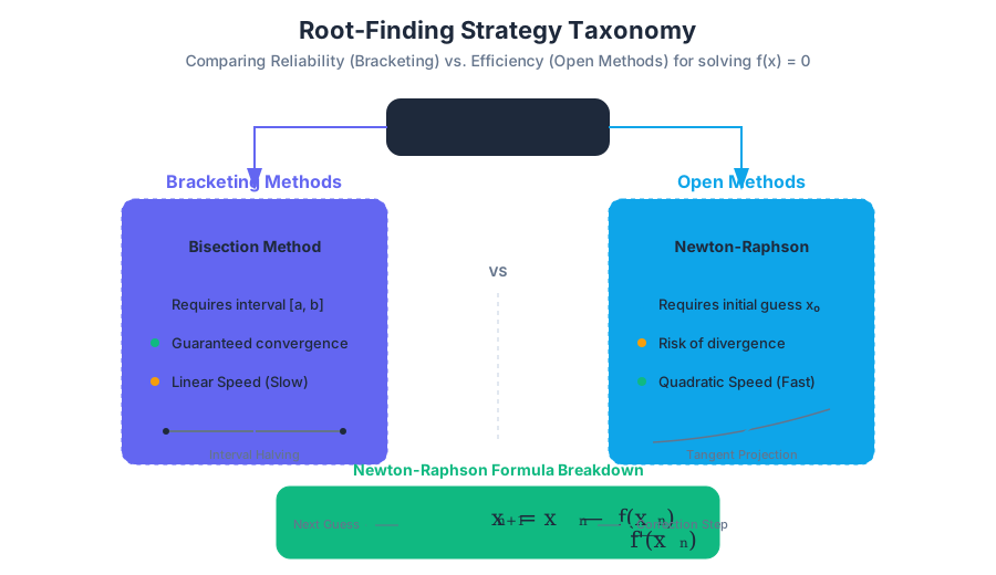
Before diving into specific algorithms, we must categorize root-finding strategies into two main families: Bracketing Methods and Open Methods. This distinction is critical for choosing the right tool for a specific engineering problem.
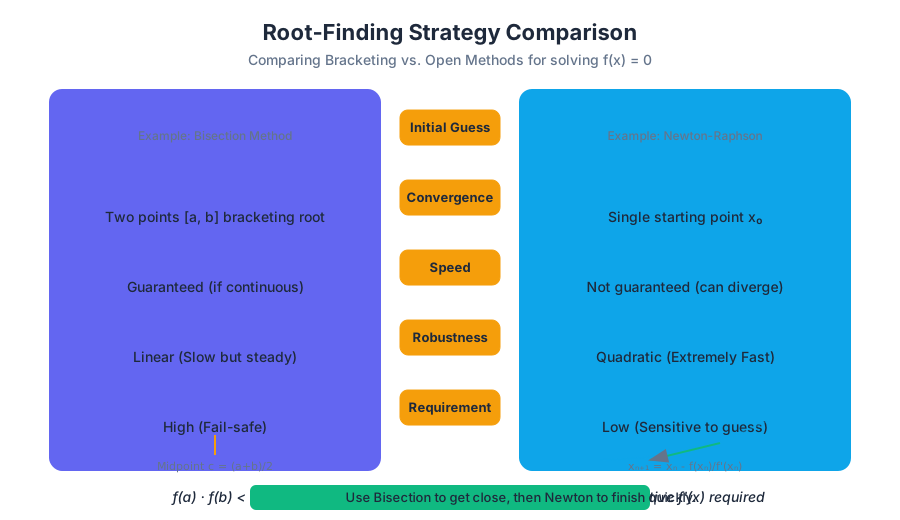
| Feature | Bracketing Methods (e.g., Bisection) | Open Methods (e.g., Newton, Secant) |
|---|---|---|
| Initial Guess | Requires two points that bracket the root. | Requires one or two starting points, not necessarily bracketing. |
| Convergence | Guaranteed to converge if $f(x)$ is continuous. | Not guaranteed; can diverge or oscillate. |
| Speed | Slow (Linear convergence). | Fast (Quadratic or Superlinear convergence). |
| Robustness | High; very reliable. | Low; sensitive to the initial guess. |
| Requirements | $f(a)$ and $f(b)$ must have opposite signs. | May require derivatives ($f'(x)$). |
The Intermediate Value Theorem (IVT): If $f(x)$ is a continuous function on the interval $[a, b]$ and $f(a)$ and $f(b)$ have opposite signs (i.e., $f(a) \cdot f(b) < 0$), then there exists at least one root $c$ within the interval $(a, b)$ such that $f(c) = 0$.
Bisection Method
The Bisection Method is the numerical equivalent of a binary search. It is a bracketing method that systematically halves an interval to home in on a root.
1. What it is
The Bisection Method is an iterative algorithm that relies on the Intermediate Value Theorem. By repeatedly dividing an interval in half and selecting the sub-interval where the sign change occurs, the method "traps" the root.
2. Why it matters
It is the "fail-safe" of root-finding. While slow, it is mathematically guaranteed to converge to a root if the function is continuous and a valid bracket is provided. It is often used to get a "close enough" guess before switching to a faster method like Newton-Raphson.
3. How it works
- Start with an interval $[a, b]$ such that $f(a) \cdot f(b) < 0$.
- Calculate the midpoint $c = \frac{a+b}{2}$.
- Evaluate $f(c)$.
- Update the interval:
- If $f(a) \cdot f(c) < 0$, the root is in $[a, c]$. Set $b = c$.
- If $f(c) \cdot f(b) < 0$, the root is in $[c, b]$. Set $a = c$.
- If $f(c) = 0$, $c$ is the exact root.
- Repeat until the interval width $|b - a|$ is less than a predefined tolerance $\epsilon$.
4. Concrete Example: Solving $f(x) = x^2 - 3$
Let's find $\sqrt{3}$ using the interval $[1, 2]$. Note that $f(1) = -2$ and $f(2) = 1$.
| Iteration | $a$ | $b$ | $c$ (Midpoint) | $f(c)$ | Sign Change? |
|---|---|---|---|---|---|
| 1 | 1.000 | 2.000 | 1.500 | -0.750 | $[1.5, 2.0]$ |
| 2 | 1.500 | 2.000 | 1.750 | 0.0625 | $[1.5, 1.75]$ |
| 3 | 1.500 | 1.750 | 1.625 | -0.359 | $[1.625, 1.75]$ |
| 4 | 1.625 | 1.750 | 1.6875 | -0.152 | $[1.6875, 1.75]$ |
5. Convergence Analysis
The error at step $n$ is bounded by: $$E_n = \frac{b-a}{2^n}$$ To achieve a specific tolerance $\epsilon$, the number of iterations $n$ required is: $$n > \frac{\ln((b-a)/\epsilon)}{\ln(2)}$$ This confirms linear convergence: each iteration adds roughly 0.301 digits of precision (since $\log_{10}(2) \approx 0.301$).
Newton-Raphson Method
The Newton-Raphson Method (often just called Newton's Method) is the gold standard for speed in root-finding, provided you have access to the function's derivative.
1. What it is
Newton's Method is an open method that uses the tangent line of the function at a current guess to predict the location of the root.
2. Why it matters
It converges quadratically, meaning the number of correct digits roughly doubles with each iteration. In high-performance computing, this efficiency is vital.
3. How it works (Derivation)
Consider the Taylor Series expansion of $f(x)$ around the current guess $x_n$: $$f(x_{n+1}) = f(x_n) + f'(x_n)(x_{n+1} - x_n) + \dots$$ Setting $f(x_{n+1}) = 0$ and ignoring higher-order terms, we solve for $x_{n+1}$: $$0 = f(x_n) + f'(x_n)(x_{n+1} - x_n)$$ $$x_{n+1} = x_n - \frac{f(x_n)}{f'(x_n)}$$
4. Implementation in Python
As mentioned in the course materials, Python's simple syntax makes it ideal for implementing these iterative loops.
def newton_method(f, df, x0, tol, max_iter):
    """
    Newton-Raphson for root finding.
    f: function, df: derivative, x0: initial guess
    """
    x = x0
    for i in range(max_iter):
        fx = f(x)
        dfx = df(x)

        if abs(dfx) < 1e-12:
            print("Derivative too small; method fails.")
            return None

        x_new = x - fx / dfx

        if abs(x_new - x) < tol:
            print(f"Converged in {i+1} iterations.")
            return x_new

        x = x_new
    return x

# Example: f(x) = x^2 - 2, f'(x) = 2x
root = newton_method(lambda x: x**2 - 2, lambda x: 2*x, 1.5, 1e-7, 100)
print(f"Root: {root}")
5. Common Pitfalls
- Divergence: If the initial guess is far from the root, the method may fly off to infinity.
- Stationary Points: If $f'(x_n) = 0$, the formula involves division by zero.
- Cycles: The method can get stuck in an infinite loop between two values.
- Multiple Roots: If a root has multiplicity $m > 1$ (e.g., $f(x) = (x-1)^2$), convergence drops from quadratic to linear.
Secant Method
The Secant Method is a clever modification of Newton's Method designed for cases where the derivative $f'(x)$ is unknown or computationally expensive to calculate.
1. What it is
Instead of using the instantaneous slope (the derivative), the Secant Method uses the slope of a line passing through the two most recent points.
2. Why it matters
It provides a "middle ground" between Bisection and Newton. It is faster than Bisection but doesn't require the symbolic derivative needed for Newton.
3. How it works
We approximate the derivative $f'(x_n)$ using the finite difference: $$f'(x_n) \approx \frac{f(x_n) - f(x_{n-1})}{x_n - x_{n-1}}$$ Substituting this into the Newton-Raphson formula gives the Secant update rule: $$x_{n+1} = x_n - f(x_n) \frac{x_n - x_{n-1}}{f(x_n) - f(x_{n-1})}$$
4. Comparison of Convergence
The Secant Method has a convergence rate of $\phi \approx 1.618$ (the Golden Ratio). It is superlinear, meaning it is faster than Bisection (rate = 1) but slower than Newton (rate = 2).
| Method | Convergence Rate ($p$) | Formula for Error $e_{n+1}$ |
|---|---|---|
| Bisection | 1 (Linear) | $e_{n+1} = 0.5 e_n$ |
| Secant | 1.618 (Superlinear) | $e_{n+1} = C e_n^{1.618}$ |
| Newton | 2 (Quadratic) | $e_{n+1} = C e_n^2$ |
5. Concrete Example: Solving $f(x) = x^2 - 2$
Initial guesses: $x_0 = 1, x_1 = 2$.
- $f(1) = -1, f(2) = 2$
- $x_2 = 2 - 2 \frac{2 - 1}{2 - (-1)} = 2 - 2(1/3) = 1.3333$
- $f(1.3333) = -0.2222$
- $x_3 = 1.3333 - (-0.2222) \frac{1.3333 - 2}{-0.2222 - 2} = 1.4000$
Convergence Analysis and Stopping Criteria
In practical numerical computing, we rarely find the exact root. Instead, we stop when our approximation is "good enough." Choosing the right stopping criterion is essential to avoid infinite loops or premature termination.
Types of Errors
- Absolute Error: $|x_{n+1} - x_n| < \epsilon$
- Relative Error: $\frac{|x_{n+1} - x_n|}{|x_{n+1}|} < \epsilon$ (Preferred when the root magnitude is unknown).
- Function Tolerance: $|f(x_n)| < \epsilon$ (Ensures the result is actually a "zero").
Comparison Table: Method Selection Matrix
| If your function is... | And you have... | Use this method: |
|---|---|---|
| Highly unpredictable | Only an interval | Bisection |
| Smooth and differentiable | A symbolic derivative | Newton-Raphson |
| Smooth but complex | No symbolic derivative | Secant |
| A black box | No derivative, limited evals | Brent's Method (Hybrid) |
Pro-Tip: In professional libraries (like
scipy.optimize), a hybrid approach called Brent's Method is often used. It combines the reliability of Bisection with the speed of inverse quadratic interpolation, switching between them based on the behavior of the function.
Practical Pitfalls in Root-Finding
Even with robust algorithms, numerical root-finding can fail in subtle ways.
1. The "Near-Zero" Derivative
In Newton's method, if $f'(x)$ is very small, the step size $\Delta x = f(x)/f'(x)$ becomes massive, shooting the next guess far away from the local region. This is common near local minima or maxima.
2. Multiple Roots
If a function touches the x-axis without crossing it (e.g., $f(x) = x^2$), Bisection will fail because there is no sign change. Newton's method will work but will lose its quadratic convergence, slowing down to linear.
3. Ill-Conditioned Problems
If the function is very "flat" near the root, a large range of $x$ values may satisfy $|f(x)| < \epsilon$. This leads to high uncertainty in the root's location.
4. Floating Point Precision
As discussed in the introductory Python materials, computers have finite precision. If your tolerance $\epsilon$ is smaller than the machine epsilon (typically $\sim 10^{-16}$ for doubles), your loop may never terminate.
Summary of Workflow
To solve a nonlinear equation $f(x)=0$ in a real-world scenario:
- Plot the function to identify the approximate location of roots and check for discontinuities.
- Check for derivatives. If $f'(x)$ is easy to compute, use Newton.
- Establish a bracket. If you need guaranteed convergence, start with Bisection.
- Implement stopping criteria. Use a combination of relative error and function tolerance.
- Validate. Plug the result back into $f(x)$ to ensure it is sufficiently close to zero.
Source Materials
Study Numerical Analysis and Computational Methods on Lykke
This course page is free to open: signed out, you can read its first two sections, and signing in, on any plan, opens the rest. The free Lykke Chrome extension syncs your own Canvas courses, so ChatGPT, Claude and Muse can answer from your classes and deadlines. It only reads Canvas.
Add the free extensionSign in to open every sectionAll sections of Numerical Analysis and Computational Methods · Browse more course pages