From the free course Numerical Analysis and Computational Methods on Lykke
Linear Systems and Direct Solvers
Key concepts: Gaussian Elimination · LU Decomposition · Pivoting Strategies · Matrix Norms
Techniques for solving systems of linear equations using matrix decomposition and elimination.
Linear Systems and Direct Solvers
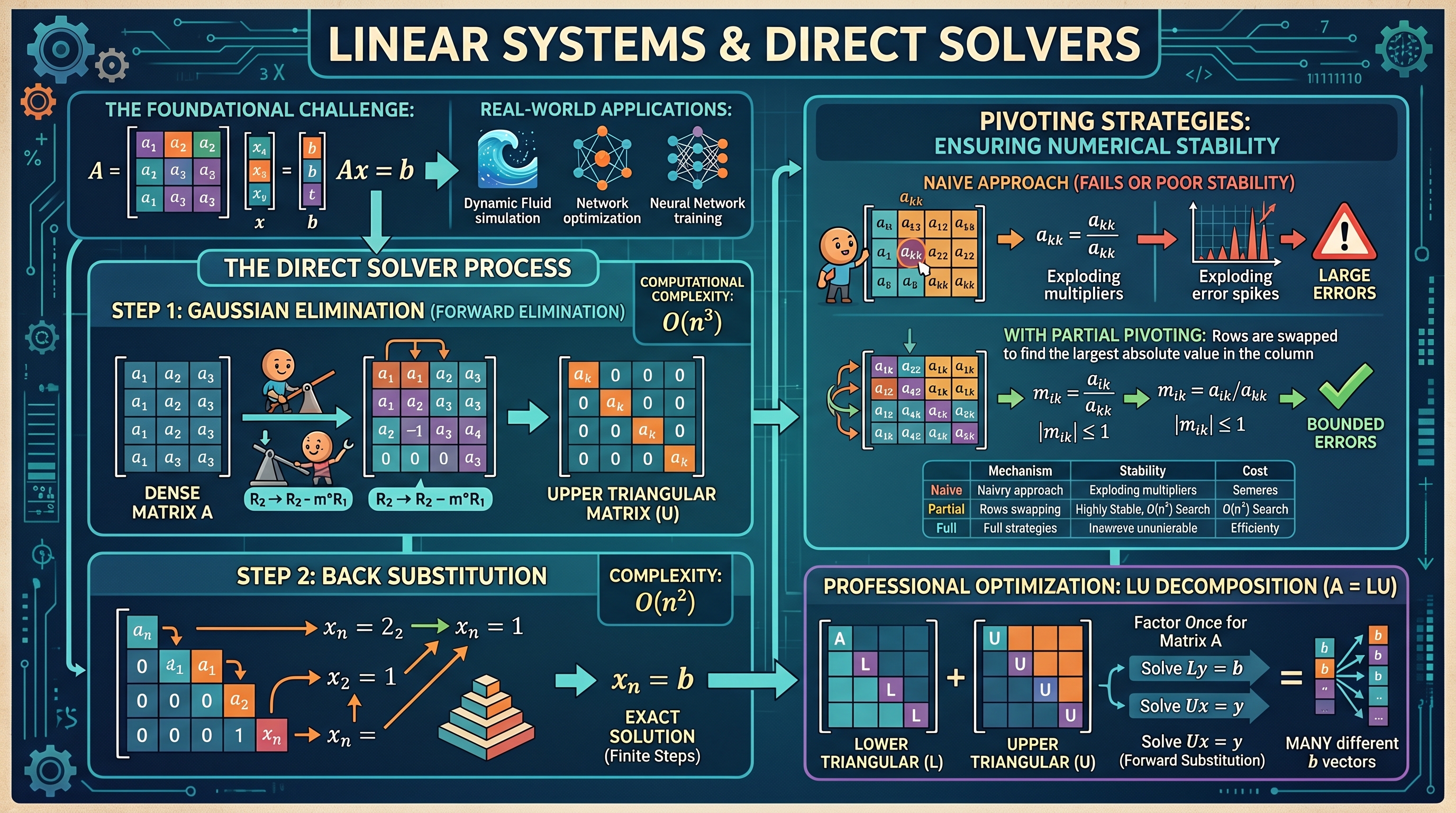
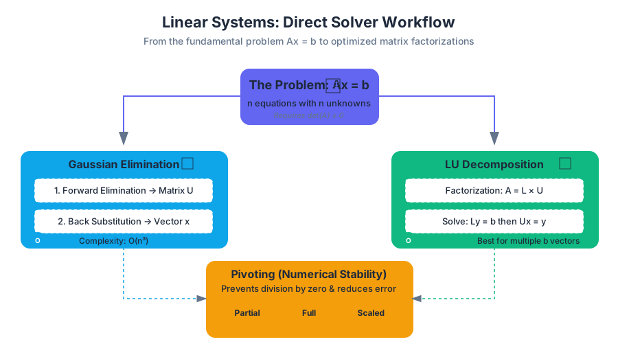
The problem of solving a system of linear equations, represented compactly as $Ax = b$, is the foundational challenge of numerical linear algebra. Whether we are simulating fluid dynamics, optimizing a supply chain, or training a neural network, we eventually encounter a set of linear constraints that must be resolved. In this deep dive, we explore Direct Solvers—algorithms that, in the absence of round-off error, provide an exact solution in a finite number of steps.
The Fundamental Problem: $Ax = b$
At its core, a linear system consists of $n$ equations with $n$ unknowns. We represent this using a matrix $A \in \mathbb{R}^{n \times n}$, a solution vector $x \in \mathbb{R}^n$, and a constant vector $b \in \mathbb{R}^n$.
Definition: A system $Ax = b$ has a unique solution if and only if the matrix $A$ is non-singular. This is equivalent to saying that the determinant $\det(A) \neq 0$, the rank of $A$ is $n$, or that the columns of $A$ are linearly independent.
While Cramer’s Rule provides a theoretical formula for $x$, its computational complexity of $O((n+1)!)$ makes it unusable for any system larger than $3 \times 3$. Direct solvers like Gaussian Elimination and LU Decomposition provide the efficiency required for real-world applications.
Gaussian Elimination: The Foundation
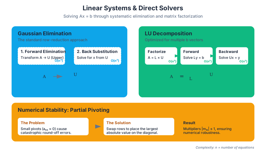
Gaussian Elimination (GE) is the systematic process of applying elementary row operations to transform a dense matrix $A$ into an Upper Triangular Matrix $U$. Once in this form, the system can be solved easily using Back Substitution.
How it Works: The Algorithm
The process is divided into two main phases:
- Forward Elimination: For each column $k$ from $1$ to $n-1$, we eliminate the entries below the diagonal element $a_{kk}$ (the pivot) in all rows $i > k$. This is done by subtracting a multiple $m_{ik} = a_{ik} / a_{kk}$ of row $k$ from row $i$.
- Back Substitution: Starting from the last equation (which now has only one unknown), we solve for $x_n$, then substitute it back into the $(n-1)$-th equation to find $x_{n-1}$, and so on.
Computational Complexity
The efficiency of GE is measured in Floating Point Operations (FLOPs).
| Phase | Operation Count (Approx.) | Complexity Class |
|---|---|---|
| Forward Elimination | $\frac{2}{3}n^3$ | $O(n^3)$ |
| Back Substitution | $n^2$ | $O(n^2)$ |
| Total | $\frac{2}{3}n^3 + n^2$ | $O(n^3)$ |
Worked Example: Gaussian Elimination
Solve the following system: $$ \begin{aligned} 2x_1 + x_2 + x_3 &= 8 \ -3x_1 - x_2 + 2x_3 &= -11 \ -2x_1 + x_2 + 2x_3 &= -3 \end{aligned} $$
Step 1: Forward Elimination
- Pivot $a_{11} = 2$.
- Eliminate $a_{21}$: $R_2 \leftarrow R_2 - (-3/2)R_1 \implies R_2 \leftarrow R_2 + 1.5R_1$. New $R_2 = [0, 0.5, 3.5, 1]$.
- Eliminate $a_{31}$: $R_3 \leftarrow R_3 - (-2/2)R_1 \implies R_3 \leftarrow R_3 + 1R_1$. New $R_3 = [0, 2, 3, 5]$.
Step 2: Eliminate below new pivot $a_{22} = 0.5$
- $R_3 \leftarrow R_3 - (2/0.5)R_2 \implies R_3 \leftarrow R_3 - 4R_2$.
- New $R_3 = [0, 0, -11, 1]$.
Step 3: Back Substitution
- $-11x_3 = 1 \implies x_3 = -1/11$.
- $0.5x_2 + 3.5(-1/11) = 1 \implies x_2 = 2.636...$
- Substitute $x_2, x_3$ into $R_1$ to find $x_1$.
Pivoting Strategies: Ensuring Stability
A naive implementation of Gaussian Elimination fails if a pivot $a_{kk}$ is zero (division by zero) or performs poorly if $a_{kk}$ is very small relative to other elements (leading to massive round-off errors).
Partial Pivoting
To solve this, we use Partial Pivoting. Before eliminating a column, we look at all elements in the current column $k$ at or below the diagonal. We find the element with the largest absolute value and swap its row with the current pivot row.
Theorem: Partial pivoting ensures that the multipliers $m_{ik}$ used in elimination always satisfy $|m_{ik}| \le 1$. This bounds the growth of numerical errors and prevents division by zero in non-singular matrices.
Comparison of Pivoting Techniques
| Strategy | Mechanism | Pros | Cons |
|---|---|---|---|
| Naive (None) | Use $a_{kk}$ as is. | Fastest (no searches). | Unstable; fails on zero pivots. |
| Partial | Swap rows to get max $\vert a_{ik}\vert $ in column. | Highly stable; standard in libraries. | Slight overhead of $O(n^2)$ search. |
| Full | Swap rows AND columns for max $\vert a_{ij}\vert $. | Most stable possible. | Expensive $O(n^3)$ search; rarely worth it. |
| Scaled Partial | Pivot based on relative size in row. | Better for poorly scaled rows. | More complex logic. |
LU Decomposition: The Professional's Choice
In many engineering contexts, we need to solve $Ax = b$ for many different $b$ vectors while $A$ remains the same (e.g., a structural frame under different loading conditions). Gaussian Elimination would require re-processing $A$ every time. LU Decomposition solves this by factoring $A$ into two triangular matrices.
The Factorization
We decompose $A$ such that: $$A = LU$$ Where:
- $L$ is a Lower Triangular matrix (with 1s on the diagonal).
- $U$ is an Upper Triangular matrix (the result of GE).
Solving with LU
Once we have $L$ and $U$, solving $Ax = b$ becomes a two-step process:
- Solve $Ly = b$ using Forward Substitution.
- Solve $Ux = y$ using Back Substitution.
Since both $L$ and $U$ are triangular, these steps only take $O(n^2)$ time. The expensive $O(n^3)$ work is done once to find $L$ and $U$.
Python Implementation of LU Decomposition
The following code demonstrates a basic LU decomposition using the Doolittle algorithm.
import numpy as np

def lu_decomposition(A):
    n = len(A)
    L = np.eye(n) # Identity matrix for L
    U = A.copy().astype(float)

    for k in range(n):
        for i in range(k + 1, n):
            # Calculate multiplier
            factor = U[i, k] / U[k, k]
            L[i, k] = factor
            # Eliminate entries in U
            U[i, k:] -= factor * U[k, k:]

    return L, U

# Example usage
A_mat = np.array([[2, 1, 1],
                  [4, 3, 3],
                  [8, 7, 9]])

L, U = lu_decomposition(A_mat)
print("L:\n", L)
print("U:\n", U)
print("Verification (L @ U):\n", L @ U)
Matrix Norms and Condition Numbers
How do we know if our solution $x$ is "good"? In numerical computing, small changes in input (due to measurement error or floating-point precision) can lead to large changes in output. We quantify this using Norms and the Condition Number.
Vector and Matrix Norms
A norm $|x|$ is a measure of the "length" or "size" of a vector or matrix.
| Norm Type | Vector Formula ($\Vert x\Vert $) | Matrix Definition ($\Vert A\Vert $) |
|---|---|---|
| $L_1$ Norm | $\sum \vert x_i\vert $ | Max absolute column sum. |
| $L_2$ (Euclidean) | $\sqrt{\sum x_i^2}$ | Spectral norm (max singular value). |
| $L_\infty$ Norm | $\max \vert x_i\vert $ | Max absolute row sum. |
The Condition Number $\kappa(A)$
The condition number measures how sensitive the solution $x$ is to perturbations in $b$.
$$\kappa(A) = |A| \cdot |A^{-1}|$$
- If $\kappa(A) \approx 1$, the matrix is Well-Conditioned.
- If $\kappa(A) \gg 1$, the matrix is Ill-Conditioned.
The Rule of Thumb: If $\kappa(A) = 10^k$, you may lose up to $k$ digits of precision in your solution $x$ beyond what is lost to standard floating-point round-off.
Special Cases and Optimized Solvers
Not all matrices require the full $O(n^3)$ treatment. Exploiting matrix structure can lead to significant speedups.
1. Tridiagonal Matrices
In many differential equation solvers, the matrix $A$ only has non-zero entries on the main diagonal and the two adjacent diagonals. The Thomas Algorithm (a simplified version of GE) solves these systems in $O(n)$ time.
2. Symmetric Positive Definite (SPD) Matrices
If $A = A^T$ and $x^T Ax > 0$ for all $x \neq 0$, we can use Cholesky Decomposition: $$A = LL^T$$ This is twice as fast as LU decomposition and numerically more stable, as it does not require pivoting.
3. Summary of Direct Methods
| Method | Matrix Requirement | Complexity | Best Use Case |
|---|---|---|---|
| Gaussian Elimination | General Non-singular | $O(n^3)$ | Single solve, general $A$. |
| LU Decomposition | General Non-singular | $O(n^3)$ | Multiple $b$ vectors for same $A$. |
| Cholesky | SPD | $\frac{1}{3}n^3$ | Optimization, Physics simulations. |
| Thomas Algorithm | Tridiagonal | $O(n)$ | 1D Heat/Wave equations. |
Common Pitfalls and Troubleshooting
- The "Singular" Trap: If your solver returns
NaNorInf, check the determinant. If $\det(A) = 0$, the system has no solution or infinite solutions. Direct solvers require a non-singular matrix. - Ignoring Pivoting: Never use naive Gaussian Elimination for large systems. Floating-point errors accumulate rapidly; always use a library that implements partial pivoting (like
scipy.linalg.solve). - The Inverse Mistake: A common novice mistake is calculating $x = A^{-1}b$ by explicitly finding $A^{-1}$.
- Why it's bad: Computing $A^{-1}$ is more expensive than LU decomposition and usually less numerically stable. Never invert a matrix to solve a linear system. Use a solver.
- Scaling Issues: If the entries in your matrix differ by many orders of magnitude (e.g., $10^{-10}$ and $10^{10}$), the condition number will explode. Normalize your equations before solving.
Source Materials
Study Numerical Analysis and Computational Methods on Lykke
This course page is free to open: signed out, you can read its first two sections, and signing in, on any plan, opens the rest. The free Lykke Chrome extension syncs your own Canvas courses, so ChatGPT, Claude and Muse can answer from your classes and deadlines. It only reads Canvas.
Add the free extensionSign in to open every sectionAll sections of Numerical Analysis and Computational Methods · Browse more course pages