From the free course Numerical Analysis and Computational Methods on Lykke
Iterative Methods for Linear Systems
Key concepts: Jacobi Method · Gauss-Seidel Method · Convergence Criteria · Sparse Matrices
Alternative approaches for solving very large or sparse linear systems where direct methods are computationally expensive.
Iterative Methods for Linear Systems
In the realm of numerical linear algebra, we are often tasked with solving the fundamental equation $Ax = b$. For small systems, direct methods like Gaussian Elimination or LU Decomposition are the gold standard, providing an exact solution (modulo floating-point error) in a predictable number of steps. However, as we transition into the domains of big data, structural engineering, and fluid dynamics, we encounter matrices with millions—or even billions—of rows. In these high-dimensional spaces, direct methods collapse under the weight of $O(n^3)$ computational complexity and massive memory requirements.
This is where Iterative Methods become indispensable. Unlike direct methods that attempt to reach the solution in one multi-step "sweep," iterative methods start with an initial guess $x^{(0)}$ and generate a sequence of approximations $x^{(1)}, x^{(2)}, \dots, x^{(k)}$ that converge toward the true solution.
The Motivation for Iteration: Direct vs. Iterative
To understand why a professor or senior engineer would choose an iterative approach over a direct one, we must look at the trade-offs in computational "budget." Direct methods are robust but "heavy." Iterative methods are "light" but require specific conditions to ensure they don't wander off into divergence.
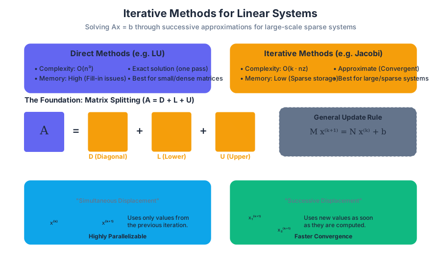
| Feature | Direct Methods (e.g., LU, QR) | Iterative Methods (e.g., Jacobi, GS) |
|---|---|---|
| Complexity | Typically $O(n^3)$ | $O(k \cdot n^2)$ or $O(k \cdot nz)$ where $nz$ is non-zeros |
| Memory Usage | High (suffers from "fill-in") | Low (can operate on sparse formats) |
| Exactness | Exact (ignoring round-off) | Approximate (controlled by tolerance $\epsilon$) |
| Suitability | Small to medium dense systems | Large, sparse systems |
| Stopping Point | Must complete all steps | Can stop early if "good enough" |
Key Insight: In many engineering applications, we do not need 16 decimal places of accuracy. If an iterative method can get within $10^{-6}$ of the solution in a few dozen iterations, it is vastly more efficient than waiting hours for a direct solver to finish.
The Mathematical Foundation: Matrix Splitting
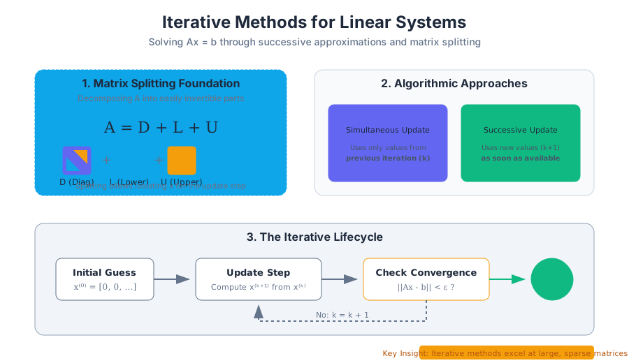
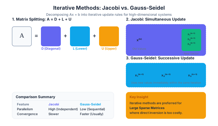
Most classical iterative methods rely on a technique called Matrix Splitting. We decompose the matrix $A$ into parts that are easy to invert. Specifically, we represent $A$ as:
$$A = D + L + U$$
Where:
- $D$ is the Diagonal matrix containing $a_{ii}$.
- $L$ is the Strictly Lower Triangular matrix (elements below the diagonal).
- $U$ is the Strictly Upper Triangular matrix (elements above the diagonal).
By rearranging $Ax = b$ as $(D + L + U)x = b$, we can isolate different components to create an update rule.
The Jacobi Method
What it is
The Jacobi Method is the simplest iterative algorithm for solving a system of linear equations. It is a "simultaneous displacement" method, meaning it calculates all components of the new vector $x^{(k+1)}$ using only the values from the previous vector $x^{(k)}$.
How it works
For each row $i$, we solve the equation for the variable $x_i$:
$$x_i^{(k+1)} = \frac{1}{a_{ii}} \left( b_i - \sum_{j \neq i} a_{ij} x_j^{(k)} \right)$$
In matrix form, this is expressed as: $$x^{(k+1)} = D^{-1} (b - (L + U)x^{(k)})$$
Python Implementation
As noted in the course materials, Python's syntax is straightforward. We don't need to declare types; we simply implement the logic using loops or NumPy.
def jacobi(A, b, x0, tolerance, max_iterations):
    n = len(b)
    x = x0.copy()
    x_new = x0.copy()

    for k in range(max_iterations):
        for i in range(n):
            sum_j = 0
            for j in range(n):
                if i != j:
                    sum_j = sum_j + A[i][j] * x[j]
            x_new[i] = (b[i] - sum_j) / A[i][i]

        # Check for convergence (L2 norm)
        diff = 0
        for i in range(n):
            diff += (x_new[i] - x[i])**2
        if (diff**0.5) < tolerance:
            return x_new

        x = x_new.copy()
    return x
Concrete Example
Consider the system: $4x_1 + x_2 = 5$ $x_1 + 3x_2 = 4$
With initial guess $x^{(0)} = [0, 0]^T$:
- Iteration 1:
- $x_1^{(1)} = (5 - (1)(0)) / 4 = 1.25$
- $x_2^{(1)} = (4 - (1)(0)) / 3 = 1.33$
- Iteration 2:
- $x_1^{(2)} = (5 - (1)(1.33)) / 4 = 0.9175$
- $x_2^{(2)} = (4 - (1)(1.25)) / 3 = 0.9166$
The values will eventually converge to the true solution $x = [1, 1]^T$.
The Gauss-Seidel Method
What it is
The Gauss-Seidel Method is an evolution of Jacobi. It observes that as soon as we calculate $x_1^{(k+1)}$, it is likely a better approximation than $x_1^{(k)}$. Therefore, we should use it immediately to calculate $x_2^{(k+1)}$, and so on. This is known as the "successive displacement" method.
How it works
The scalar formula incorporates the "new" values as they become available:
$$x_i^{(k+1)} = \frac{1}{a_{ii}} \left( b_i - \sum_{j < i} a_{ij} x_j^{(k+1)} - \sum_{j > i} a_{ij} x_j^{(k)} \right)$$
In matrix form: $$(D + L)x^{(k+1)} = b - Ux^{(k)}$$ $$x^{(k+1)} = (D + L)^{-1} (b - Ux^{(k)})$$
Comparison of Update Logic
| Method | Data Usage | Parallelism | Convergence Speed |
|---|---|---|---|
| Jacobi | Uses only "old" data from step $k$ | High (all $x_i$ can be computed at once) | Generally slower |
| Gauss-Seidel | Uses "new" data as soon as it's computed | Low (sequential dependency) | Generally faster |
Python Implementation
Note how Gauss-Seidel is actually easier to implement in a memory-efficient way because we can update the vector x in-place.
def gauss_seidel(A, b, x0, tolerance, max_iterations):
    n = len(b)
    x = x0.copy()

    for k in range(max_iterations):
        x_old = x.copy()
        for i in range(n):
            sum_j = 0
            for j in range(n):
                if i != j:
                    sum_j = sum_j + A[i][j] * x[j] # Uses current x[j]
            x[i] = (b[i] - sum_j) / A[i][i]

        # Convergence check
        error = sum((x[i] - x_old[i])**2 for i in range(n))**0.5
        if error < tolerance:
            return x
    return x
Convergence Criteria
Not every matrix $A$ will converge using these methods. If the matrix is "poorly behaved," the iterations might spiral out to infinity.
Strictly Diagonally Dominant (SDD) Matrices
The most common sufficient condition for convergence is Strict Diagonal Dominance.
Definition: A matrix $A$ is Strictly Diagonally Dominant if, for every row $i$, the magnitude of the diagonal element is greater than the sum of the magnitudes of all other elements in that row: $$|a_{ii}| > \sum_{j \neq i} |a_{ij}|$$
If $A$ is SDD, both Jacobi and Gauss-Seidel are guaranteed to converge for any initial guess $x^{(0)}$.
The Spectral Radius
For a more general analysis, we look at the Iteration Matrix $M$. Any iterative method can be written as: $$x^{(k+1)} = Mx^{(k)} + c$$
- For Jacobi: $M_J = -D^{-1}(L+U)$
- For Gauss-Seidel: $M_{GS} = -(D+L)^{-1}U$
Theorem: The iterative method converges if and only if the Spectral Radius $\rho(M) < 1$. The spectral radius is the largest absolute eigenvalue of $M$. The smaller $\rho(M)$, the faster the convergence.
| Condition | Impact on Jacobi | Impact on Gauss-Seidel |
|---|---|---|
| SDD | Guaranteed Convergence | Guaranteed Convergence |
| Symmetric Positive Definite | Not Guaranteed | Guaranteed Convergence |
| $\rho(M) \ge 1$ | Divergence | Divergence |
Sparse Matrices and Efficiency
In modern computing, we rarely store large matrices as 2D arrays. A 1,000,000 x 1,000,000 matrix would require 8 Terabytes of RAM if stored as doubles. However, in many fields, most of these entries are zero. This is a Sparse Matrix.
Why Iterative Methods Win here
Direct methods like LU decomposition create "fill-in." Even if $A$ is sparse, $L$ and $U$ might be dense, destroying our memory efficiency. Iterative methods, however, only require the ability to perform a Matrix-Vector Multiplication ($Ax$).
We can store $A$ in formats like Compressed Sparse Row (CSR):
values: Only the non-zero numbers.column_indices: Which column each value belongs to.row_pointers: Where each row starts in thevaluesarray.
Complexity Comparison
If a matrix has $n$ rows and an average of $z$ non-zero entries per row:
- Direct Method: $O(n^3)$
- Iterative Method (per iteration): $O(n \cdot z)$
If $z$ is small (e.g., $z=10$ for a 3D mesh), the iterative method is effectively $O(n)$ per iteration. This scalability is why Google's PageRank (an eigenvector problem solved iteratively) and weather simulations are possible.
Variations and Extensions: SOR
While Gauss-Seidel is faster than Jacobi, we can accelerate it even further using Successive Over-Relaxation (SOR).
SOR introduces a relaxation parameter $\omega$ (omega): $$x_i^{(k+1)} = (1 - \omega)x_i^{(k)} + \frac{\omega}{a_{ii}} \left( b_i - \sum_{j < i} a_{ij} x_j^{(k+1)} - \sum_{j > i} a_{ij} x_j^{(k)} \right)$$
- If $\omega = 1$: We have standard Gauss-Seidel.
- If $1 < \omega < 2$: We are "over-relaxing," pushing the solution faster toward the limit. This is used to speed up convergence.
- If $0 < \omega < 1$: We are "under-relaxing," which can help stabilize a system that would otherwise diverge.
Common Pitfalls and Troubleshooting
- Zero on the Diagonal: Both Jacobi and Gauss-Seidel involve dividing by $a_{ii}$. If any diagonal element is zero, the method fails immediately. A common fix is Pivoting (swapping rows) before starting the iteration.
- Slow Convergence: If $\rho(M)$ is very close to 1 (e.g., 0.999), the method may take thousands of iterations to converge. In such cases, preconditioning or switching to Krylov subspace methods (like Conjugate Gradient) is necessary.
- The "False Convergence" Trap: If your tolerance is too loose, or if the solution is changing very slowly, the algorithm might stop before it reaches the actual solution. Always check the Residual $r = b - Ax^{(k)}$ to ensure the solution actually satisfies the original equation.
- Ordering Matters: In Gauss-Seidel, the order in which you update $x_i$ affects the results and the rate of convergence. In some specialized hardware (like GPUs), "Red-Black" ordering is used to allow for partial parallelism.
Summary of Iterative Workflow
- Analyze the Matrix: Check for sparsity and diagonal dominance.
- Choose a Method: Jacobi for parallel systems, Gauss-Seidel for sequential speed, or SOR for optimized performance.
- Set Parameters: Define a starting guess $x^{(0)}$ (often all zeros), a tolerance $\epsilon$, and a maximum iteration count to prevent infinite loops.
- Iterate: Update $x$ until the change between steps (or the residual) is below $\epsilon$.
- Validate: Plug the result back into $Ax = b$ to verify accuracy.
Source Materials
Study Numerical Analysis and Computational Methods on Lykke
This course page is free to open: signed out, you can read its first two sections, and signing in, on any plan, opens the rest. The free Lykke Chrome extension syncs your own Canvas courses, so ChatGPT, Claude and Muse can answer from your classes and deadlines. It only reads Canvas.
Add the free extensionSign in to open every sectionAll sections of Numerical Analysis and Computational Methods · Browse more course pages