From the free course Numerical Analysis and Computational Methods on Lykke
Introduction and Python for Numerical Computing
Key concepts: Python Syntax · Variable Types · Arithmetic Operators · Operator Precedence · Computational Applications
Foundational course logistics and an introduction to Python programming as the primary tool for numerical implementation.
Introduction and Python for Numerical Computing
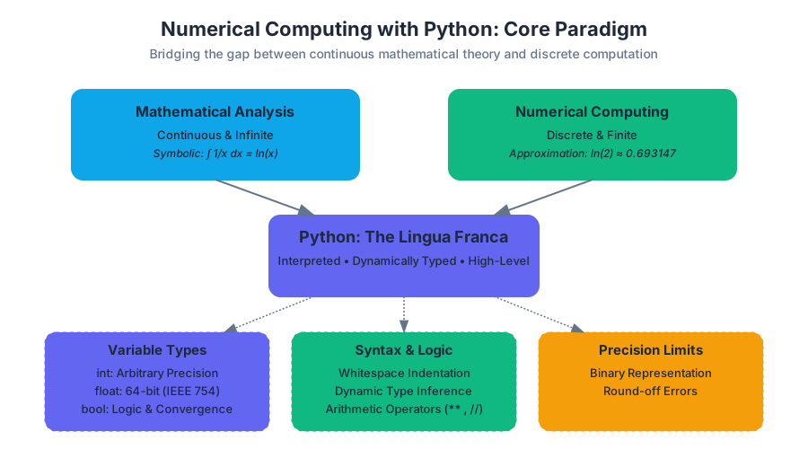
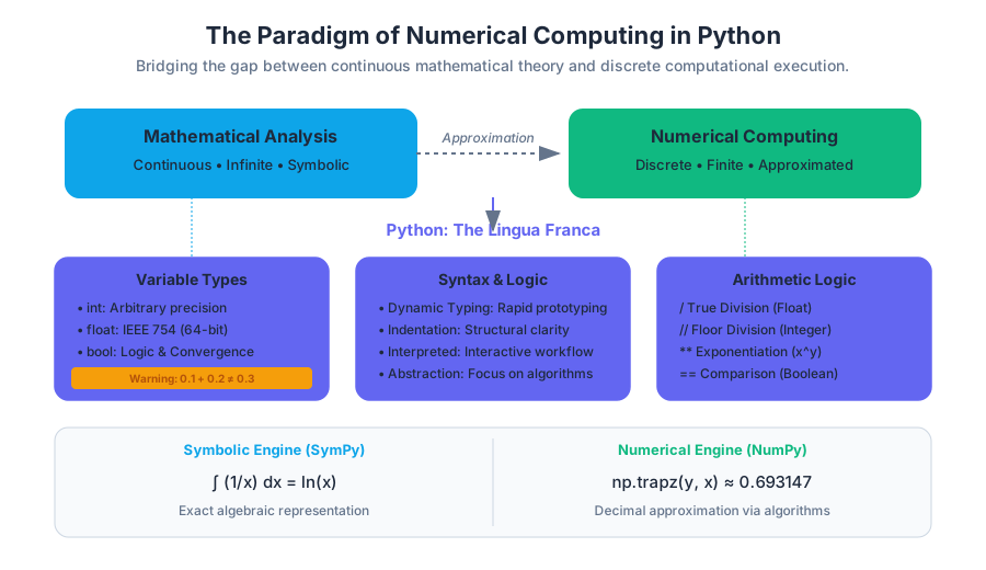
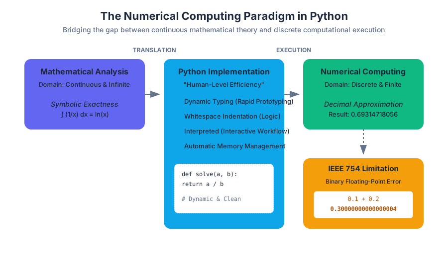
Numerical analysis is the study of algorithms that use numerical approximation for the problems of mathematical analysis. In the modern era, this discipline is inseparable from the computational tools used to implement it. While theoretical mathematics often deals with the infinite and the continuous, computers are finite and discrete. This fundamental tension—representing the continuous within the discrete—is the heart of numerical computing.
Python has emerged as the lingua franca of this field. Its rise is not due to raw execution speed, but rather its "human-level" efficiency: the speed with which a researcher can translate a complex mathematical model into a functioning program. This section explores the foundational syntax and logic of Python, specifically through the lens of numerical application.
The Paradigm of Numerical Computing
Numerical computing differs from symbolic computing. While a symbolic engine (like Mathematica or SymPy) might tell you that the integral of $1/x$ is $\ln(x)$, a numerical engine (like the ones we will build in Python) provides a decimal approximation, such as $0.693147$.
Definition: Numerical Analysis The branch of mathematics that designs and analyzes algorithms for obtaining numerical solutions to problems that involve continuous variables. These problems arise throughout the natural sciences, social sciences, engineering, medicine, and business.
In this course, we utilize Python because it abstracts away low-level memory management, allowing us to focus on the stability and convergence of our algorithms. However, this abstraction requires a deep understanding of how Python handles data types and operations to avoid "silent" errors in precision.
Python Syntax and the Interpreter Environment
Python is an interpreted, high-level, dynamically typed language. Unlike compiled languages such as C++ or Fortran, Python code is executed line-by-line by the Python Interpreter. This allows for an interactive workflow, which is essential when testing numerical convergence or visualizing data.
The Role of Indentation
In most programming languages, curly braces {} or keywords like begin/end define blocks of code. Python uses whitespace indentation. This is not merely a stylistic choice but a syntactic requirement.
# A simple example of Python's clean syntax
def calculate_area(radius):
    pi = 3.141592653589793
    area = pi * (radius ** 2)
    return area

print(calculate_area(5))
Implicit vs. Explicit Declaration
One of Python's most powerful features for rapid prototyping is dynamic typing. You do not need to declare that a variable is an integer or a float; the interpreter infers the type at runtime based on the value assigned.
| Feature | Python Approach | Benefit for Numerical Work |
|---|---|---|
| Typing | Dynamic | Faster implementation of formulas |
| Memory | Automatic Garbage Collection | Focus on logic, not memory leaks |
| Syntax | Minimalist (No semicolons) | Reduces visual noise in complex equations |
| Libraries | Extensive (NumPy, SciPy) | Access to optimized C-level routines |
Variable Types and Memory Representation
In numerical computing, the type of a variable dictates the precision of your result. Python handles several standard types, but for our purposes, int, float, and bool are the most critical.
Integers (int)
Python 3 integers have arbitrary precision. This means they can grow as large as your computer's memory allows, avoiding the "overflow" errors common in 32-bit or 64-bit integer types in other languages.
Floating-Point Numbers (float)
In Python, float corresponds to double-precision (64-bit) binary floating-point numbers, following the IEEE 754 standard.
Key Insight: The Floating-Point Limitation Because computers represent numbers in base-2 (binary), certain base-10 decimals cannot be represented exactly. For example,
0.1 + 0.2in Python results in0.30000000000000004. In numerical analysis, managing these "round-off errors" is a primary concern.
Booleans (bool)
Representing True or False, booleans are the backbone of conditional logic and convergence criteria (e.g., "Stop the loop when the error is less than $10^{-6}$").
Arithmetic Operators and Mathematical Logic
Python provides a robust set of operators to perform calculations. Understanding the distinction between different division types is particularly important for algorithm design.
Basic Arithmetic
The standard operators follow expected mathematical conventions:
+(Addition)-(Subtraction)*(Multiplication)/(True Division): Always returns a float.//(Floor Division): Divides and rounds down to the nearest whole number.%(Modulo): Returns the remainder of the division.**(Exponentiation): $x^y$ is written asx ** y.
Comparison and Logical Operators
These operators evaluate expressions to return a Boolean value, which is essential for implementing piecewise functions or iterative loops.
| Operator | Description | Example |
|---|---|---|
== |
Equal to | 5 == 5 (True) |
!= |
Not equal to | 5 != 3 (True) |
> |
Greater than | 5 > 10 (False) |
< |
Less than | 2 < 4 (True) |
and |
Logical AND | True and False (False) |
or |
Logical OR | True or False (True) |
not |
Logical NOT | not True (False) |
Worked Example: The Quadratic Formula
To see these operators in action, consider the calculation of the discriminant in the quadratic formula $D = b^2 - 4ac$:
# Coefficients for x^2 + 5x + 6 = 0
a = 1
b = 5
c = 6

# Calculating the discriminant
discriminant = b**2 - 4*a*c

# Using comparison logic
if discriminant > 0:
    root1 = (-b + discriminant**0.5) / (2*a)
    root2 = (-b - discriminant**0.5) / (2*a)
    print(f"Roots are real: {root1}, {root2}")
elif discriminant == 0:
    root = -b / (2*a)
    print(f"One real root: {root}")
else:
    print("Roots are complex")
Operator Precedence: The Hierarchy of Evaluation
In numerical computing, a single misplaced parenthesis can lead to catastrophic errors in simulation. Python follows a specific hierarchy, often summarized by the acronym PEMDAS (Parentheses, Exponents, Multiplication/Division, Addition/Subtraction).
The Precedence Table
The following table ranks operators from highest precedence (evaluated first) to lowest (evaluated last).
| Rank | Operator | Description |
|---|---|---|
| 1 | () |
Parentheses (Grouping) |
| 2 | ** |
Exponentiation |
| 3 | +x, -x, ~x |
Unary plus, minus, bitwise NOT |
| 4 | *, /, //, % |
Multiplication, Division, Floor Div, Modulo |
| 5 | +, - |
Addition, Subtraction |
| 6 | <<, >> |
Bitwise shifts |
| 7 | & |
Bitwise AND |
| 8 | ^ |
Bitwise XOR |
| 9 | | |
Bitwise OR |
| 10 | ==, !=, >, <, etc. |
Comparisons |
| 11 | not |
Logical NOT |
| 12 | and |
Logical AND |
| 13 | or |
Logical OR |
Case Study: Evaluating Complex Expressions
Consider the expression for a Gaussian distribution: $$f(x) = \frac{1}{\sigma\sqrt{2\pi}} e^{-\frac{1}{2}(\frac{x-\mu}{\sigma})^2}$$
In Python, without proper attention to precedence, this could be written incorrectly. Let's break down the correct implementation:
import math

x = 1.0
mu = 0.0
sigma = 1.0

# Correct implementation using precedence and parentheses
fx = (1 / (sigma * math.sqrt(2 * math.pi))) * math.exp(-0.5 * ((x - mu) / sigma)**2)
Common Pitfall: Writing 1 / sigma * math.sqrt(...) would result in $(1/\sigma) \cdot \sqrt{\dots}$ instead of $1 / (\sigma \cdot \sqrt{\dots})$. Always use parentheses to make the denominator explicit.
Computational Applications: Why We Compute
Numerical computing is not an abstract exercise; it is the engine of modern engineering. When analytical (exact) solutions are impossible to find, we turn to numerical approximations.
1. Space Exploration and Orbital Mechanics
Calculating the trajectory of a spacecraft requires solving systems of differential equations that have no closed-form solution. By discretizing time into small steps ($\Delta t$), we can use Python to predict the position of a rover on Mars with millimeter precision.
2. Autonomous Vehicles
Self-driving cars process LIDAR and camera data in real-time. This involves massive matrix multiplications and optimization algorithms (like Gradient Descent) implemented using the very operators discussed above. The speed and accuracy of these numerical calculations are literally a matter of life and death.
3. Financial Modeling
The Black-Scholes model for option pricing or Monte Carlo simulations for risk assessment rely on generating millions of random numerical outcomes to find an expected value.
| Application | Numerical Method Used | Role of Python |
|---|---|---|
| Weather Prediction | Fluid Dynamics Simulations | Handling large multi-dimensional arrays |
| Structural Engineering | Finite Element Analysis (FEA) | Solving massive systems of linear equations |
| Machine Learning | Backpropagation / Optimization | Efficiently updating weights via partial derivatives |
Common Pitfalls in Numerical Python
As you begin implementing algorithms, be wary of these common "gotchas" that can derail your computations.
- Integer Division in Older Versions: In Python 2,
5/2resulted in2. In Python 3, it correctly results in2.5. However, if you specifically need an integer, you must use5 // 2. - Floating Point Equality: Never use
==to compare two floats. Because of round-off errors,0.1 + 0.2 == 0.3will returnFalse. Instead, check if the difference is smaller than a tiny tolerance (epsilon):abs(a - b) < 1e-9. - Mutable Default Arguments: While not strictly numerical, assigning a list as a default argument in a function can lead to shared state across function calls, corrupting numerical data.
- Shadowing Built-in Names: Avoid naming your variables
sum,min,max, ortype, as these are built-in Python functions. Doing so will "shadow" the function, making it inaccessible later in your script.
Summary of the Computational Pipeline
The journey from a mathematical concept to a numerical result follows a structured pipeline.
- Mathematical Modeling: Define the continuous equations (e.g., Newton's Laws).
- Discretization: Convert the continuous model into a discrete form suitable for a computer.
- Algorithm Design: Choose a method (e.g., Euler's method, Newton-Raphson).
- Implementation: Write the Python code using correct variables, operators, and precedence.
- Verification: Test against known solutions and check for numerical stability.
By mastering the basic syntax and understanding the underlying logic of Python's arithmetic, you lay the groundwork for the more complex iterative methods that define numerical analysis.
Source Materials
Study Numerical Analysis and Computational Methods on Lykke
This course page is free to open: signed out, you can read its first two sections, and signing in, on any plan, opens the rest. The free Lykke Chrome extension syncs your own Canvas courses, so ChatGPT, Claude and Muse can answer from your classes and deadlines. It only reads Canvas.
Add the free extensionSign in to open every sectionAll sections of Numerical Analysis and Computational Methods · Browse more course pages