From the free course Motion Planning with Graphs of Convex Sets on Lykke
Convex Relaxations and Tightness
Key concepts: Convex Relaxation · Integrality Gap · Strong Formulations · Dual Problems
Deep dive into why GCS is computationally efficient and how it avoids the exponential complexity of traditional solvers.
Convex Relaxations and Tightness
In the landscape of modern robotics and motion planning, the "holy grail" has long been an algorithm that combines the global optimality of discrete graph search with the dynamic feasibility of continuous trajectory optimization. Historically, these two worlds were separated by a computational chasm: discrete search (like A*) handles combinatorial complexity but struggles with high-dimensional dynamics, while continuous optimization (like SQP) handles dynamics but gets trapped in local minima created by obstacles. The Graphs of Convex Sets (GCS) framework, as introduced by Russ Tedrake and his team, bridges this chasm by reformulating motion planning as a convex optimization problem over a graph. Central to the success of this approach is the concept of Convex Relaxations and their Tightness—the mathematical property that allows us to solve NP-hard combinatorial problems with the efficiency of simple convex programs.
The Combinatorial Challenge: Mixed-Integer Programming (MIP)
To understand why convex relaxations are necessary, we must first acknowledge the inherent difficulty of motion planning around obstacles. When a robot encounters an obstacle, it faces a binary choice: go left or go right. In mathematical terms, this is an "either/or" constraint, which is non-convex. The standard way to model such decisions is through Mixed-Integer Programming (MIP). In a MIP, some variables are constrained to be integers (usually binary, $y \in {0, 1}$), representing discrete choices, while others are continuous ($x \in \mathbb{R}^n$), representing positions or velocities.
Definition: Mixed-Integer Program (MIP) A MIP is an optimization problem of the form: $$\min_{x, y} f(x, y)$$ subject to: $$g(x, y) \leq 0$$ $$x \in \mathbb{R}^n, y \in {0, 1}^m$$ Where $y$ represents the discrete decisions (e.g., "Am I in region A or region B?") and $x$ represents the continuous state.
While MIPs are incredibly expressive, they are generally NP-hard. Solving them typically requires a "Branch and Bound" approach, which explores a search tree of binary decisions. In the worst case, the number of branches grows exponentially with the number of obstacles, making real-time motion planning for complex environments computationally prohibitive.
| Feature | Mixed-Integer Programming (MIP) | Standard Nonlinear Optimization |
|---|---|---|
| Decision Type | Discrete + Continuous | Continuous Only |
| Global Optimality | Guaranteed (given enough time) | Not Guaranteed (local minima) |
| Complexity | Exponential (NP-hard) | Polynomial (usually) |
| Obstacle Handling | Exact (via binary variables) | Heuristic (via penalty functions) |
Defining Convex Relaxation
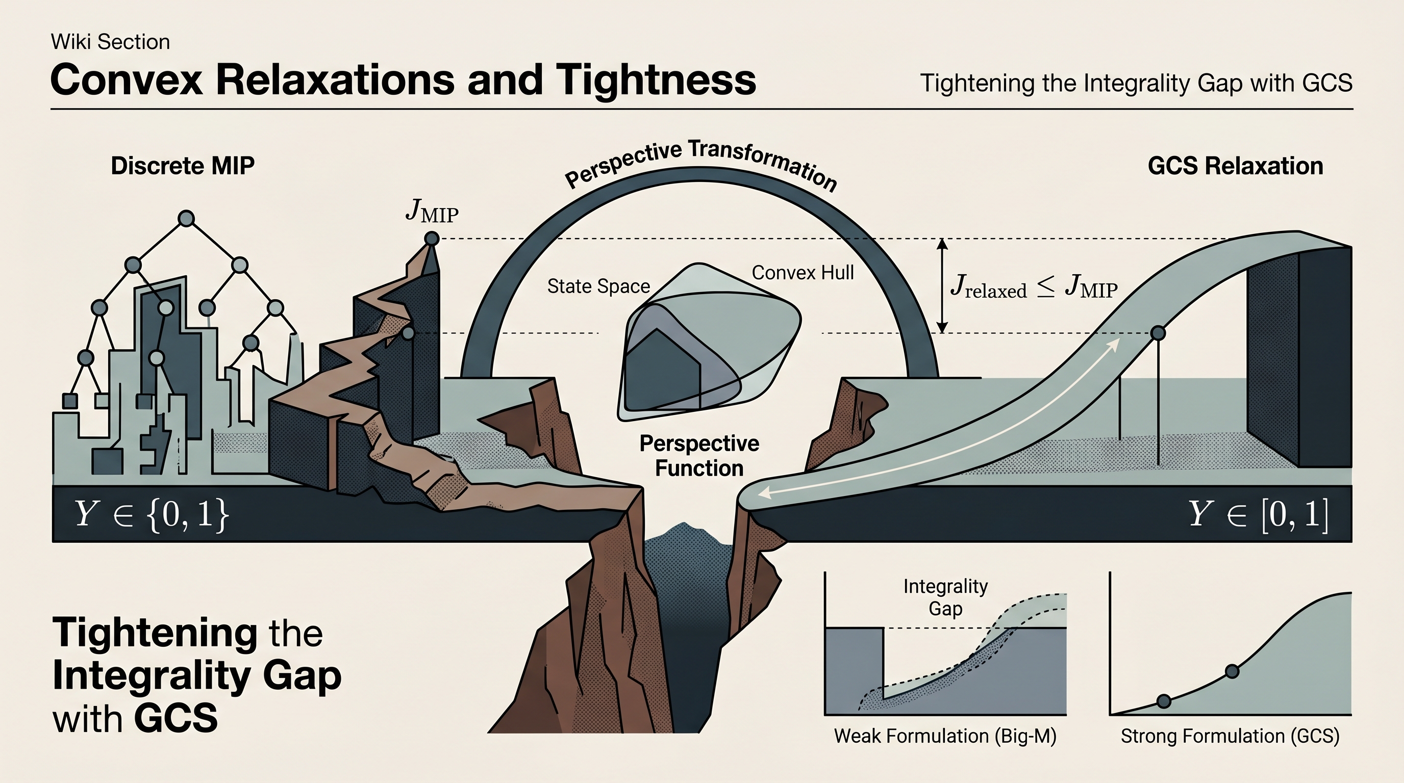
A Convex Relaxation is the process of taking a hard, non-convex problem and replacing it with a simpler, convex one that "contains" the original. In the context of GCS, we relax the binary constraint $y \in {0, 1}$ to a continuous interval constraint $y \in [0, 1]$. This transformation turns a combinatorial search into a continuous optimization problem that can be solved in polynomial time using interior-point methods.
Mathematically, if the original feasible set is $S$, the relaxation seeks a convex set $\hat{S}$ such that $S \subseteq \hat{S}$. The goal is to find the "tightest" possible $\hat{S}$—the one that most closely hugs the original non-convex set. If the relaxation is perfectly tight, the optimal solution to the relaxed problem will naturally land on an integer value (0 or 1), even though it was allowed to be anything in between.
The Integrality Gap
The quality of a relaxation is measured by the Integrality Gap. This is the difference between the objective value of the optimal integer solution ($J_{MIP}$) and the objective value of the relaxed solution ($J_{relaxed}$). Since the relaxed problem is less constrained, its optimal value is always less than or equal to the true integer optimum: $$J_{relaxed} \leq J_{MIP}$$
A gap of zero implies that the relaxation is tight. In GCS, the objective is to formulate the graph search such that the integrality gap is zero or near-zero, allowing the solver to find the globally optimal path without ever explicitly "branching" on the binary variables.
Strong Formulations and the Perspective Function
Not all relaxations are created equal. A "weak" formulation might satisfy the constraints but result in a large integrality gap, leading the solver to produce "fuzzy" solutions where a robot is 50% in one region and 50% in another. To achieve Tightness, GCS utilizes what is known in the optimization community as a Strong Formulation.
The secret to the GCS "strength" is the use of the Perspective Function. When we associate a continuous variable $x$ (like a position) with a binary variable $y$ (representing whether we are in a specific convex set $X$), we don't just say $x \in X$ if $y=1$. Instead, we use a higher-dimensional representation: $$x \in yX$$ Where $yX$ is the scaling of the set $X$ by the factor $y$. If $y=1$, the constraint is $x \in X$. If $y=0$, the constraint collapses to $x=0$.
The Mathematical Derivation
If a convex set is defined by the inequalities $Ax \leq b$, the perspective of that set is defined by: $$A(x/y) \leq b \implies Ax \leq by$$ This transformation is crucial because the set of points $(x, y)$ satisfying $Ax \leq by$ for $y \in [0, 1]$ is itself a convex cone. By summing these perspective-based constraints across all edges and vertices in the graph, GCS creates a formulation that is the convex hull of the original shortest-path problem.
| Formulation Type | Mechanism | Tightness | Solver Performance |
|---|---|---|---|
| Big-M Formulation | $x \leq M \cdot y$ | Weak | Slow convergence, large gaps |
| Convex Hull (GCS) | $Ax \leq by$ | Strong | Fast convergence, often zero gap |
| Penalty Methods | $\lambda \cdot \text{dist}(x, X)$ | Very Weak | Prone to local minima |
The Dual Problem: Potentials and Lower Bounds
In optimization, every primal problem (the one we want to solve) has a Dual Problem. For GCS, the dual problem provides deep insights into why the relaxation is so effective. In the context of a graph, the dual variables can be interpreted as Potentials at each vertex.
If we are looking for the shortest path from a start vertex $s$ to a goal vertex $t$, the dual problem is essentially trying to find the largest possible lower bound on the cost-to-go. In a standard graph, this is equivalent to the Bellman equation. In GCS, because each node is a convex set, the dual variables represent "cost-to-go functions" over those sets.
Key Insight: The Dual as a Certificate The dual problem provides a "certificate" of optimality. If the value of the dual objective matches the value of the primal objective, we have proof that we have found the global optimum. Because the GCS relaxation is so tight, the dual bound is often extremely high, which allows the solver to prune large sections of the graph that cannot possibly contain the optimal solution.
Dual Variables in GCS:
- $\phi_v$: The potential at vertex $v$.
- $\lambda_{uv}$: The dual variables associated with the edges.
- Interpretation: The dual problem maximizes the potential at the start node subject to the constraint that the potential difference between nodes cannot exceed the cost of the edge connecting them.
Why GCS is "Tight" in Practice
One of the most surprising results presented by Russ Tedrake is that for many motion planning problems, the GCS relaxation is exactly tight. This means the solver returns an integer solution ($y=0$ or $y=1$) directly, without any rounding or branching.
This tightness stems from the fact that the GCS formulation is the convex hull of the flow constraints on a graph. In classical network flow theory, the "Shortest Path Problem" on a graph is known to have a Totally Unimodular (TU) constraint matrix. TU matrices have the magical property that their vertices are always integers. While the addition of convex set constraints (the "continuous" part) breaks pure TU, the "Strong Formulation" using perspective functions preserves much of this structure, keeping the integrality gap at or near zero for a wide class of problems.
Factors Influencing Tightness:
- Set Overlap: If convex sets overlap significantly, the relaxation remains strong.
- Cost Function: Linear or convex quadratic costs (like squared distance) tend to preserve tightness.
- Graph Topology: Cycles in the graph can sometimes introduce gaps, but GCS handles this by enforcing flow conservation.
Worked Example: Navigating a "U-Shaped" Obstacle
Consider a robot that must move from $(0,0)$ to $(10,10)$ but must pass around a large U-shaped obstacle. A standard nonlinear optimizer would likely drive the robot into the "pocket" of the U and get stuck in a local minimum.
- Decomposition: We decompose the free space into three overlapping convex sets: $X_1$ (left of the U), $X_2$ (right of the U), and $X_3$ (above the U).
- Graph Construction: We create a graph where vertices are these sets. Edges exist where sets overlap.
- MIP Formulation: We define binary variables $y_{12}, y_{23}$, etc., to represent the path taken.
- Relaxation: We relax $y \in [0, 1]$ and apply the perspective transformation to the dynamics.
- Execution: The solver (e.g., Mosek or Gurobi) sees a single large convex problem. It evaluates the "cost-to-go" through the left path vs. the right path simultaneously in a continuous space.
- Result: Because the formulation is tight, the solver identifies that the left path is $2.5$ units shorter and returns $y_{left}=1, y_{right}=0$. The robot follows the globally optimal trajectory without ever "seeing" the local minimum inside the U.
| Step | Action | Mathematical Tool |
|---|---|---|
| 1 | Identify Obstacles | Configuration Space Analysis |
| 2 | Partition Space | Convex Decomposition (IRIS) |
| 3 | Define Costs | Quadratic/Convex Objectives |
| 4 | Solve Relaxation | Interior-Point Method (Convex) |
| 5 | Extract Path | Integrality Check / Rounding |
Common Pitfalls and Misconceptions
While GCS and its relaxations are powerful, they are not magic. Users often encounter specific hurdles:
- The "Big-M" Trap: Many engineers attempt to implement GCS using "Big-M" constraints (e.g., $x \leq 1000 \cdot y$). This is mathematically valid but numerically disastrous. It leads to very weak relaxations and slow solver performance. Always use the perspective formulation ($Ax \leq by$).
- Non-Convex Costs: If the cost function itself is non-convex (e.g., minimizing time in a system with non-linear dynamics), the relaxation may no longer be convex. GCS requires the cost within each set to be convex.
- Over-Decomposition: While more convex sets make the approximation of free space more accurate, they also increase the number of variables in the optimization. There is a trade-off between geometric fidelity and computational speed.
- Numerical Precision: Because perspective functions involve terms like $x/y$, they can become numerically unstable as $y \to 0$. High-quality solvers handle this using specialized "rotated second-order cone" constraints to maintain stability.


Source Materials
Study Motion Planning with Graphs of Convex Sets on Lykke
This course page is free to open: signed out, you can read its first two sections, and signing in, on any plan, opens the rest. The free Lykke Chrome extension syncs your own Canvas courses, so ChatGPT, Claude and Muse can answer from your classes and deadlines. It only reads Canvas.
Add the free extensionSign in to open every sectionAll sections of Motion Planning with Graphs of Convex Sets · Browse more course pages