From the free course Motion Planning with Graphs of Convex Sets on Lykke
Applications and Performance in Robotics
Key concepts: Dynamic Feasibility · UAV Navigation · Manipulator Planning · Footstep Planning
Practical demonstrations of GCS applied to UAVs, robotic arms, and walking robots.
Applications and Performance in Robotics
The field of motion planning has long been bifurcated into two distinct philosophies: discrete graph search and continuous trajectory optimization. While graph search algorithms like A* or RRT* are excellent at navigating complex combinatorial mazes, they often struggle with high-dimensional dynamics and smoothness. Conversely, trajectory optimization excels at producing fluid, dynamically feasible motions but is notoriously susceptible to local minima in cluttered environments. Graphs of Convex Sets (GCS), as introduced by Russ Tedrake and his team, represents a unified framework that bridges this gap. By formulating the motion planning problem as a shortest path problem over a graph of convex sets, GCS provides a powerful tool for generating globally optimal, dynamically feasible trajectories for a wide array of robotic systems, from agile UAVs to complex humanoid walkers.
The GCS Framework: Unifying Discrete and Continuous Planning
At its core, GCS addresses the challenge of planning in a space that is both continuous (the robot's configuration) and discrete (the sequence of regions or "corridors" the robot must pass through). In traditional methods, one might use a graph search to find a sequence of collision-free regions and then use optimization to "smooth" a path through them. However, this decoupled approach often fails to find the true global optimum because the initial discrete choice might preclude the most efficient continuous trajectory.
Definition: Graph of Convex Sets (GCS) A GCS is a mathematical structure where nodes represent convex sets $X_i \subseteq \mathbb{R}^n$ (typically representing safe regions in configuration space) and edges represent transitions between these sets. The goal is to find a continuous trajectory $x(t)$ that starts in a source set, ends in a target set, and minimizes a cost function while remaining within the union of the sets and satisfying dynamical constraints.
The breakthrough of GCS lies in its mathematical formulation. By using the perspective function of convex costs and constraints, the problem can be formulated as a Mixed-Integer Convex Program (MICP). More importantly, the convex relaxation of this MICP is remarkably tight, often providing the exact global optimum in polynomial time for many practical robotics problems.
| Feature | Sampling-Based (RRT*) | Trajectory Opt (SQP/IPOPT) | Graphs of Convex Sets (GCS) |
|---|---|---|---|
| Optimality | Asymptotically Global | Local | Globally Optimal (or tight relaxation) |
| Dynamics | Hard to incorporate | Native support | Native support (via Bezier/Polynomials) |
| Obstacles | Handles well via collision checking | Causes local minima | Handled via convex decomposition |
| Completeness | Probabilistic | N/A | Resolution Complete / Deterministic |
The mathematical "magic" that allows GCS to remain convex involves the transformation of a trajectory segment within a set $X_i$ into a scaled version. If $f(x)$ is a convex cost, the perspective function is defined as: $$\phi(x, \lambda) = \lambda f(x/\lambda)$$ where $\lambda \in [0, 1]$ acts as a flow variable on the edge. This allows the optimizer to "decide" how much flow passes through a particular sequence of convex sets, effectively solving the combinatorial path selection and the continuous trajectory shape simultaneously.
Dynamic Feasibility in Motion Planning
A trajectory is considered dynamically feasible if it respects the physical limits of the robot, such as maximum velocity, acceleration, torque, and joint limits. In GCS, these constraints are integrated directly into the optimization problem.
Mathematical Formulation of Constraints
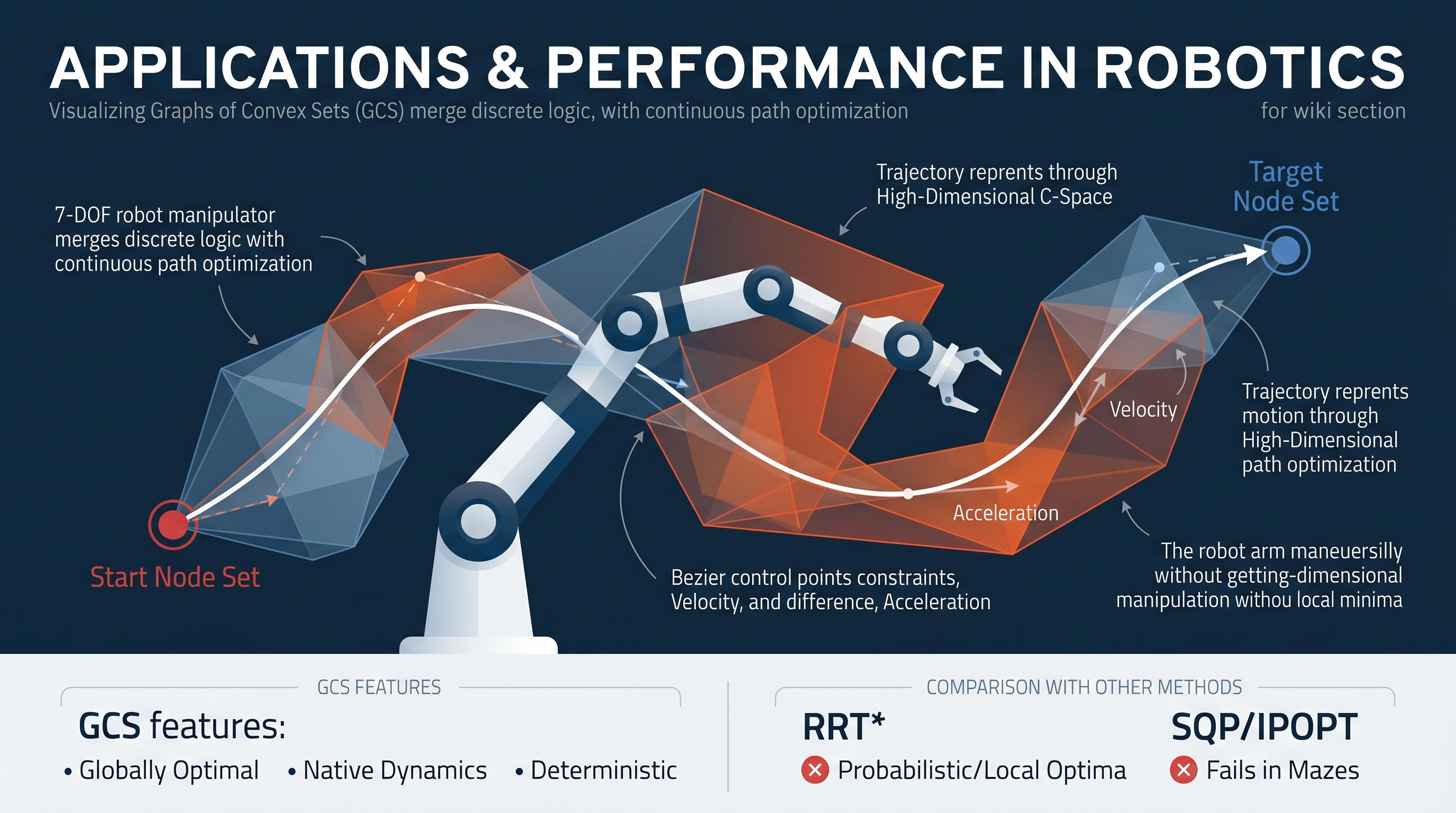
To ensure dynamic feasibility, GCS typically represents the trajectory $x(t)$ within each convex set using Bezier curves or B-splines. This choice is strategic: Bezier curves possess the convex hull property, meaning the entire curve is contained within the convex hull of its control points. If the control points are constrained to lie within a convex set $X_i$, the entire trajectory segment is guaranteed to be within $X_i$.
Dynamic constraints are applied to the derivatives of the Bezier curve. For a Bezier curve of degree $d$ with control points $P_0, \dots, P_d$, the derivative is also a Bezier curve of degree $d-1$. Thus, velocity and acceleration limits can be expressed as linear constraints on the differences between control points:
- Position: $P_j \in X_i$ for all $j$.
- Velocity: $\dot{x}(t) = d \sum (P_{j+1} - P_j) B_{j, d-1}(t) \leq v_{max}$.
- Acceleration: $\ddot{x}(t) \leq a_{max}$.
By enforcing these constraints on the control points, GCS ensures that the resulting trajectory is not just a geometric path, but a physically executable command for the robot's actuators. This eliminates the need for a separate "path tracking" or "smoothing" phase that might introduce collisions or violations of limits.
Application: UAV Navigation in Cluttered Environments
Unmanned Aerial Vehicles (UAVs) require high-speed navigation through complex environments, such as forests or indoor spaces. Traditional planners often struggle with the "narrow passage" problem or fail to account for the drone's inertia at high speeds.
The GCS Pipeline for UAVs
- Environment Decomposition: The free space is decomposed into a collection of overlapping convex polytopes using algorithms like IRIS (Iterative Regional Inflation by Semidefinite programming).
- Graph Construction: Each polytope becomes a node in the GCS. Edges are added between overlapping polytopes.
- Optimization: The GCS solver finds the minimum-time or minimum-energy trajectory that passes through a sequence of these polytopes.
In the context of a drone flying through a window, GCS doesn't just find a path through the opening; it finds the optimal approach angle and velocity that allows the drone to clear the window while minimizing its travel time. Because the optimization is global, the drone can "look ahead" and begin its banking maneuver long before it reaches the obstacle.
| Parameter | Traditional Trajectory Opt | GCS Approach |
|---|---|---|
| Initial Guess | Required (often manual/heuristic) | Not required (Global search) |
| Obstacle Avoidance | Penalty functions (Soft) | Hard constraints (Convex sets) |
| Success Rate | Low in complex mazes | High (Deterministic) |
| Compute Time | Fast (if guess is good) | Moderate (Solves relaxation) |
Application: Manipulator Planning and High-Dimensional C-Space
For a robotic arm with 7 Degrees of Freedom (DOF), the configuration space (C-space) is a 7-dimensional manifold where obstacles are complex, non-convex shapes. Standard Inverse Kinematics (IK) solvers and trajectory optimizers often get stuck in local minima—for example, the elbow of the arm might get "caught" on the wrong side of a table.
Overcoming Local Minima
GCS handles this by decomposing the C-space into convex regions. While decomposing a 7D space is computationally expensive, the IRIS algorithm can efficiently find large convex regions of free space. Once the C-space is represented as a graph of these regions, GCS can navigate the 7D maze with the same global optimality it uses for 3D drone flight.
Consider a task where a manipulator must reach into a shelf. A local optimizer might try to move the hand directly toward the goal, hitting the shelf's edge. GCS, seeing the entire graph of convex sets, recognizes that the "shortest path" in C-space involves first retracting the arm, reorienting the elbow, and then entering the shelf—a sequence of moves that is naturally discovered through the graph search component of GCS.
Self-Collision Avoidance
GCS also excels at self-collision avoidance. By representing the "safe" joint configurations (where the arm doesn't hit itself) as convex sets, the planner ensures that the arm remains in a valid state throughout the entire motion. This is a significant improvement over "sampling and checking" methods, which might miss thin regions of self-collision.
Application: Footstep Planning for Legged Robots
Walking robots present a unique challenge: the problem is inherently hybrid. There are discrete decisions (which surface to step on) and continuous decisions (the exact $(x, y, z)$ location of the foot and the trajectory of the Center of Mass).
Unified Discrete-Continuous Optimization
In traditional legged locomotion, these are often solved separately: a footstep planner finds a sequence of steps, and a whole-body controller moves the robot. GCS allows these to be solved simultaneously.
- Nodes: Represent potential stepping stones or safe terrain regions.
- Edges: Represent the reachability of the robot's leg.
- Continuous Variables: The foot position within the chosen set and the CoM trajectory.
By treating "where to step" as a path in a graph of convex sets, GCS can optimize the robot's gait for stability and speed at the same time. If a particular stepping stone requires a precarious balance, the GCS solver will either find a more stable sequence of steps or adjust the CoM trajectory to compensate, all within a single optimization loop.
| Planning Component | Discrete Variable | Continuous Variable |
|---|---|---|
| Navigation | Sequence of rooms/corridors | Path coordinates $(x, y)$ |
| Manipulation | Sequence of arm postures | Joint angles $\theta_1 \dots \theta_7$ |
| Walking | Sequence of stepping stones | Foot placement and CoM |
Performance Comparison and Benchmarking
The performance of GCS is typically measured against two benchmarks: the quality of the solution (cost) and the time to find it.
GCS vs. RRT* (Sampling-Based)
RRT* is asymptotically optimal, meaning it will eventually find the best path if given infinite time. However, in practice, RRT* paths are often "jagged" and require significant post-processing to be made smooth and dynamically feasible. GCS, by contrast, provides a smooth, feasible trajectory immediately. In benchmarks involving high-dimensional manipulators, GCS often finds a lower-cost solution in seconds than RRT* finds in minutes.
GCS vs. Mixed-Integer Programming (MIP)
Before GCS, the standard way to solve these "discrete-continuous" problems was through Big-M formulations of Mixed-Integer Programs. These are notoriously slow because their convex relaxations are "loose," forcing the solver to explore a massive branch-and-bound tree. GCS uses a stronger relaxation based on the perspective function. In many cases, the solver finds the integer-optimal solution at the very first node of the search tree, leading to speedups of several orders of magnitude.
The "Certificate of Optimality"
One of the most significant advantages of GCS is the duality gap. Because it is based on convex optimization, the solver can provide a mathematical "certificate" of how close the current solution is to the theoretical global optimum. Sampling-based planners cannot do this; they can only tell you the best path they've found so far.
Implementation Details and Complexity
While GCS is powerful, it is not a "silver bullet." Its performance depends heavily on the quality of the convex decomposition of the environment.
Computational Complexity
The size of the GCS problem scales with:
- $N$: The number of convex sets (nodes).
- $E$: The number of overlaps (edges).
- $d$: The degree of the Bezier curves (smoothness).
- $n$: The dimensionality of the configuration space.
For a fixed number of sets, the convex relaxation is a Second-Order Cone Program (SOCP) or a Semidefinite Program (SDP), both of which can be solved in polynomial time. However, as the number of sets increases, the memory requirements for the solver can become a bottleneck.
Common Pitfalls
- Poor Decomposition: If the convex sets are too small or don't overlap sufficiently, the graph may not contain the optimal path, or the solver may struggle to find flow.
- High Degree Polynomials: Using very high-degree Bezier curves to achieve extreme smoothness can lead to numerical instability in the solver.
- Non-Convex Costs: If the cost function (e.g., minimizing power consumption in a non-linear motor model) is not convex, the GCS framework requires further approximations.
Summary of Performance Metrics
The following table summarizes the typical performance profile of GCS in a standard robotic navigation task compared to other state-of-the-art methods.
| Metric | RRT* | Trajectory Opt (Local) | GCS (Relaxed) |
|---|---|---|---|
| Global Optimality | Asymptotic | No | Yes (usually) |
| Dynamic Feasibility | Post-processed | Yes | Yes |
| Solve Time (s) | 10 - 100+ | 0.1 - 1.0 | 0.5 - 5.0 |
| Reliability | Stochastic | Fails in local minima | Deterministic |
| Scalability (DOF) | High | High | Medium (due to decomposition) |
In conclusion, Graphs of Convex Sets represent a paradigm shift in robotics. By moving away from the "search then optimize" workflow and toward a "unified convex formulation," GCS allows robots to move with a level of grace and efficiency that was previously computationally prohibitive. Whether it is a drone threading a needle at 30 mph or a humanoid navigating a rubble-strewn construction site, GCS provides the mathematical backbone for the next generation of autonomous motion.


Source Materials
Study Motion Planning with Graphs of Convex Sets on Lykke
This course page is free to open: signed out, you can read its first two sections, and signing in, on any plan, opens the rest. The free Lykke Chrome extension syncs your own Canvas courses, so ChatGPT, Claude and Muse can answer from your classes and deadlines. It only reads Canvas.
Add the free extensionSign in to open every sectionAll sections of Motion Planning with Graphs of Convex Sets · Browse more course pages