From the free course Introductory Statistics on Lykke
The Chi-Square Distribution
Key concepts: Goodness-of-Fit · Test of Independence · Contingency Tables · Degrees of Freedom
Testing for relationships between categorical variables and goodness-of-fit.
The Chi-Square Distribution: Foundations of Categorical Analysis
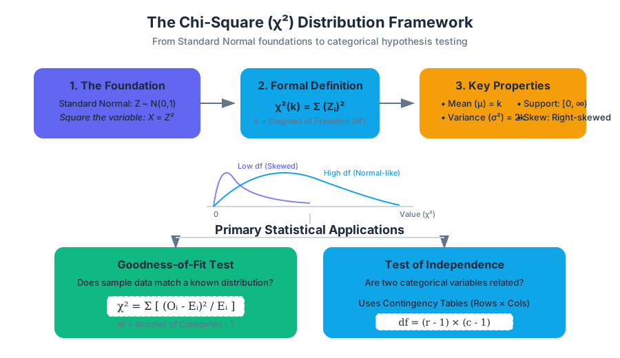
The Chi-Square ($\chi^2$) distribution is a continuous probability distribution that serves as the backbone for inferential statistics involving categorical data. While the Normal distribution governs the behavior of means, the Chi-Square distribution governs the behavior of variances and the "closeness" of observed data to theoretical models. It is not a single curve, but a family of curves defined by a single parameter: the degrees of freedom ($df$).
1. The Mathematical Foundation
At its most fundamental level, the Chi-Square distribution is derived from the Standard Normal Distribution ($Z \sim N(0,1)$). If you take a random variable from a standard normal distribution and square it, the resulting value follows a Chi-Square distribution with one degree of freedom.
Formal Definition: If $Z_1, Z_2, \dots, Z_k$ are independent, standard normal random variables, then the sum of their squares is distributed according to the Chi-Square distribution with $k$ degrees of freedom: $$X = \sum_{i=1}^{k} Z_i^2 \sim \chi^2(k)$$
Characteristics of the Distribution
The shape of the $\chi^2$ curve is highly sensitive to the value of $k$.
| Property | Description | Mathematical Expression |
|---|---|---|
| Support | The distribution is defined only for non-negative values. | $[0, \infty)$ |
| Mean | The expected value is exactly equal to the degrees of freedom. | $E[X] = k$ |
| Variance | The spread is twice the degrees of freedom. | $Var(X) = 2k$ |
| Skewness | Always right-skewed, but approaches normality as $k \to \infty$. | $\gamma_1 = \sqrt{8/k}$ |
| Mode | The peak of the density function (for $k > 2$). | $k - 2$ |
As $df$ increases, the distribution loses its sharp right skew and begins to look like a bell curve. This is an application of the Central Limit Theorem, as the distribution is essentially a sum of independent random variables.
2. Goodness-of-Fit: Testing Theoretical Models
The Chi-Square Goodness-of-Fit Test is used to determine if a sample data set matches a population with a specific distribution. It answers the question: "Is the difference between what I saw and what I expected just due to chance?"
The Mechanics
The test relies on comparing Observed frequencies ($O$) from your sample against Expected frequencies ($E$) derived from your null hypothesis ($H_0$).
- State the Hypotheses: $H_0$ states the data follows the specified distribution; $H_a$ states it does not.
- Calculate Expected Values: $E = n \times p$, where $n$ is the total sample size and $p$ is the hypothesized probability for that category.
- Compute the Test Statistic: $$\chi^2 = \sum \frac{(O_i - E_i)^2}{E_i}$$
- Determine Degrees of Freedom: $df = k - 1$, where $k$ is the number of categories.
3. The Test of Independence
While Goodness-of-Fit looks at one variable, the Test of Independence evaluates the relationship between two categorical variables. For example, is "Voting Preference" independent of "Income Level"?
Contingency Tables
Data for this test is organized into a Contingency Table (or cross-tabulation).
| Category A1 | Category A2 | Row Total | |
|---|---|---|---|
| Category B1 | Cell(1,1) | Cell(1,2) | $R_1$ |
| Category B2 | Cell(2,1) | Cell(2,2) | $R_2$ |
| Col Total | $C_1$ | $C_2$ | Grand Total ($N$) |
Calculating Expected Values in Independence Tests
In a test of independence, the expected value for any cell is calculated based on the assumption that the variables are independent (i.e., the joint probability is the product of the marginal probabilities).
Expected Cell Frequency Formula: $$E_{i,j} = \frac{(\text{Row } i \text{ Total}) \times (\text{Column } j \text{ Total})}{\text{Grand Total}}$$
Degrees of Freedom for Independence
For a table with $r$ rows and $c$ columns: $$df = (r - 1) \times (c - 1)$$ This represents the number of cells in the table that can vary independently given that the row and column totals are fixed.
Mathematical Derivation Logic
ALGORITHM ChiSquareIndependence(Matrix Observed):
    Rows = Observed.RowCount
    Cols = Observed.ColCount
    GrandTotal = Sum(Observed)

    RowTotals = [Sum(Row) for Row in Observed]
    ColTotals = [Sum(Col) for Col in Observed.Columns]

    ChiSqStat = 0
    FOR i FROM 0 TO Rows-1:
        FOR j FROM 0 TO Cols-1:
            Expected = (RowTotals[i] * ColTotals[j]) / GrandTotal
            IF Expected < 5:
                WARN "Sample size too small for reliable Chi-Square"

            Residual = Observed[i][j] - Expected
            ChiSqStat += (Residual^2) / Expected

    DF = (Rows - 1) * (Cols - 1)
    PValue = 1 - ChiSquareCDF(ChiSqStat, DF)

    RETURN ChiSqStat, DF, PValue
4. Test of Homogeneity
The Test of Homogeneity is mathematically identical to the Test of Independence but differs in its experimental design and null hypothesis.
- Independence: You take one sample from one population and see if two variables are related.
- Homogeneity: You take samples from multiple distinct populations and see if they follow the same distribution for a single variable.
| Feature | Test of Independence | Test of Homogeneity |
|---|---|---|
| Sampling | Single random sample | Multiple independent samples (one per population) |
| Question | Are Variable X and Variable Y related? | Is the distribution of Variable X the same across populations? |
| Null Hypothesis | Factors are independent. | Distributions are the same (homogeneous). |
| Calculation | $(r-1)(c-1)$ | $(r-1)(c-1)$ |
5. Practical Implementation: Real-World Usage
In modern data science, we rarely calculate these by hand. We use libraries that handle the distribution's cumulative density function (CDF) to return p-values directly.
6. Critical Assumptions and Pitfalls
The Chi-Square test is a non-parametric test in terms of population distribution (it doesn't assume the population is normal), but it is parametric in its requirement for sample sizes.
The "Rule of Five"
The most common mistake in Chi-Square analysis is applying it to small datasets. Because the $\chi^2$ distribution is a continuous approximation of a discrete process, it breaks down when expected frequencies are low.
- Cochran’s Rule: No more than 20% of the expected counts should be less than 5, and all individual expected counts should be greater than 1.
- Yates' Correction: For $2 \times 2$ tables, some statisticians apply a "continuity correction" by subtracting 0.5 from the absolute difference between $O$ and $E$. However, modern consensus often favors the Fisher's Exact Test for small samples instead.
Comparison of Methods for Categorical Data
| Method | Best Use Case | Constraint |
|---|---|---|
| Pearson's $\chi^2$ | Large samples, any table size | $E_i \ge 5$ |
| Fisher's Exact Test | $2 \times 2$ tables, small samples | Computationally expensive for large $N$ |
| G-Test | Likelihood ratio based, additive | Preferred in bioinformatics/complex models |
| McNemar's Test | Paired categorical data (before/after) | Only for dependent samples |
7. Advanced Variations: The Non-Central Chi-Square
In power analysis, we often encounter the Non-Central Chi-Square distribution. While the standard (central) Chi-Square assumes the null hypothesis is true, the non-central version describes the distribution of the test statistic when the alternative hypothesis is true.
It introduces a non-centrality parameter ($\lambda$): $$\lambda = \sum_{i=1}^{k} \mu_i^2$$ where $\mu_i$ are the means of the squared normal variables. This is crucial for calculating the Statistical Power (the probability of correctly rejecting a false null hypothesis).
8. Summary of Workflow
To perform a Chi-Square analysis effectively, follow this pipeline:
- Identify the Test Type: Is it one variable vs. a model (GoF), two variables in one population (Independence), or one variable across multiple populations (Homogeneity)?
- Verify Assumptions: Check that the data are frequencies (counts), observations are independent, and expected values are $\ge 5$.
- Construct the Table: Ensure rows and columns are mutually exclusive.
- Calculate $\chi^2$ and $df$: Use the sum of squared residuals.
- Compare to Critical Value: Use a $\chi^2$ table or software to find the p-value for the given $df$ at the desired alpha level (usually 0.05).
Study Guide: The Chi-Square Distribution
Core Concepts
- Degrees of Freedom ($df$): The primary parameter of the $\chi^2$ distribution. For GoF, it's $k-1$. For Independence, it's $(r-1)(c-1)$.
- Observed vs. Expected: The test statistic measures the cumulative deviation of actual counts ($O$) from what we would expect under the null hypothesis ($E$).
- Right-Skewed Nature: The distribution starts at zero and has a long right tail. As $df$ increases, it becomes more symmetrical.
Common Formulas
- Test Statistic: $\chi^2 = \sum \frac{(O-E)^2}{E}$
- Expected (Independence): $E = \frac{\text{Row Total} \cdot \text{Col Total}}{N}$
- Mean of Distribution: $\mu = df$
- Variance of Distribution: $\sigma^2 = 2 \cdot df$
Critical Thinking Questions
- Why can a Chi-Square statistic never be negative? (Answer: Because it is a sum of squared values).
- What happens to the p-value if the gap between Observed and Expected values increases? (Answer: The $\chi^2$ statistic increases, causing the p-value to decrease).
- If you have a $3 \times 4$ contingency table, what is the $df$? (Answer: $(3-1) \times (4-1) = 2 \times 3 = 6$).
Practical Tips
- Always use raw counts, never percentages or means, inside the Chi-Square formula.
- If your expected values are too low, consider "collapsing" categories (combining small groups) to meet the "Rule of Five."
- Remember that "Independence" does not mean "no relationship"—it specifically means no statistical association between the categorical groupings.
Source Materials
Study Introductory Statistics on Lykke
This course page is free to open: signed out, you can read its first two sections, and signing in, on any plan, opens the rest. The free Lykke Chrome extension syncs your own Canvas courses, so ChatGPT, Claude and Muse can answer from your classes and deadlines. It only reads Canvas.
Add the free extensionSign in to open every sectionAll sections of Introductory Statistics · Browse more course pages