From the free course Introductory Statistics on Lykke
The Central Limit Theorem
Key concepts: Sampling Distribution · Standard Error · Law of Large Numbers
Explaining why the normal distribution is so prevalent and how it applies to sample means.
The Central Limit Theorem (CLT)
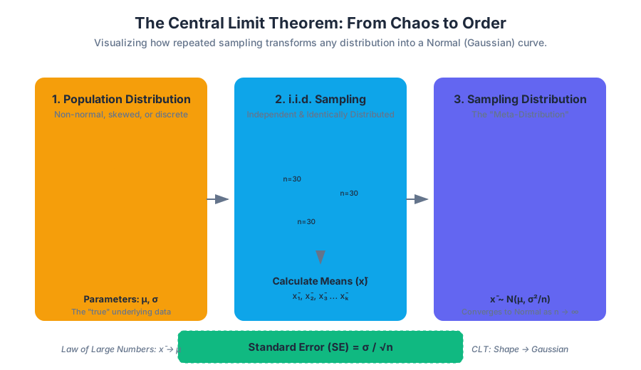
The Central Limit Theorem (CLT) is the foundational pillar of modern statistical inference. It provides the mathematical justification for why the Normal Distribution (the "Bell Curve") appears so frequently in the natural and social sciences. At its core, the CLT states that the sum (or mean) of a large number of independent, identically distributed (i.i.d.) random variables will tend toward a normal distribution, regardless of the shape of the underlying population distribution.
This theorem transforms statistics from a purely descriptive exercise into a predictive science. Without the CLT, we would be unable to calculate confidence intervals or perform hypothesis tests for complex systems where the underlying probability density function (PDF) is unknown or non-normal.
The Foundation: The Law of Large Numbers (LLN)
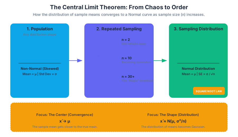
Before diving into the CLT, one must understand the Law of Large Numbers (LLN). While the CLT describes the shape of the distribution of sample means, the LLN describes where that distribution is centered.
The Law of Large Numbers: As the number of trials or observations ($n$) increases, the sample mean ($\bar{X}$) converges to the theoretical population mean ($\mu$).
There are two distinct flavors of this law that mathematicians distinguish based on the "strength" of the convergence:
- Weak Law of Large Numbers (WLLN): States that for any non-zero margin, the probability that the sample mean differs from the population mean approaches zero as $n \to \infty$. This is convergence in probability.
- Strong Law of Large Numbers (SLLN): States that the sample mean converges to the population mean "almost surely." This means the probability that the sequence of means converges to $\mu$ is equal to 1.
LLN vs. CLT: A Critical Distinction
| Feature | Law of Large Numbers (LLN) | Central Limit Theorem (CLT) |
|---|---|---|
| Primary Focus | Convergence of the mean value. | Convergence of the distribution shape. |
| Result | $\bar{X} \to \mu$ | $\bar{X} \approx \mathcal{N}(\mu, \sigma^2/n)$ |
| Utility | Guarantees stability of long-term averages. | Enables probabilistic inference and error estimation. |
| Requirement | Finite first moment (Mean exists). | Finite second moment (Variance exists). |
The Mechanics of the Sampling Distribution
To understand the CLT, we must first define the Sampling Distribution. This is not the distribution of the raw data itself, but a "meta-distribution" of a statistic (like the mean) calculated from repeated samples of size $n$.
Imagine a population of 1 million people. If we take a sample of 100 people and calculate their average height, that single average is one data point in our sampling distribution. If we repeat this process 10,000 times, the resulting histogram of those 10,000 averages will form the sampling distribution.
Properties of the Sampling Distribution of the Mean
As $n$ increases, the sampling distribution exhibits three predictable behaviors:
- Center: The mean of the sampling distribution ($\mu_{\bar{x}}$) is equal to the mean of the population ($\mu$).
- Spread: The standard deviation of the sampling distribution, known as the Standard Error (SE), decreases as the sample size increases.
- Shape: The distribution becomes increasingly Gaussian (Normal), even if the population is heavily skewed or discrete.
The Standard Error: Quantifying Precision
The Standard Error (SE) is the standard deviation of the sampling distribution. It measures how much the sample mean is expected to vary from the true population mean.
Definition: The Standard Error of the Mean (SEM) is calculated as: $$SE = \frac{\sigma}{\sqrt{n}}$$ Where $\sigma$ is the population standard deviation and $n$ is the sample size.
This formula reveals the Square Root Law: to cut your measurement error in half, you must quadruple your sample size. This is a fundamental constraint in experimental design and polling.
Comparison of Standard Deviation and Standard Error
| Metric | Symbol | Description | Relationship to $n$ |
|---|---|---|---|
| Standard Deviation | $\sigma$ | Measures the dispersion of individual data points in the population. | Independent of $n$. |
| Sample Std Dev | $s$ | An estimate of $\sigma$ derived from a single sample. | Becomes a better estimate as $n$ grows. |
| Standard Error | $SE$ | Measures the dispersion of sample means around the true mean. | Inversely proportional to $\sqrt{n}$. |
Formal Statement of the Central Limit Theorem
In its most common form (the Lindeberg-Lévy CLT), the theorem is stated as follows:
Suppose ${X_1, X_2, \dots, X_n}$ is a sequence of i.i.d. random variables with $E[X_i] = \mu$ and $Var[X_i] = \sigma^2 < \infty$. As $n$ approaches infinity, the random variables $\sqrt{n}(\bar{X}_n - \mu)$ converge in distribution to a normal distribution $\mathcal{N}(0, \sigma^2)$:
$$\bar{X}_n \xrightarrow{d} \mathcal{N}\left(\mu, \frac{\sigma^2}{n}\right)$$
Mathematical Derivation via Characteristic Functions
To truly understand why the CLT works, we look at Characteristic Functions ($\phi_X(t)$). The characteristic function of a random variable is the Fourier transform of its probability density function. A key property is that the characteristic function of the sum of independent variables is the product of their individual characteristic functions.
The Proof Sketch
- Let $Z_n = \frac{\sum X_i - n\mu}{\sigma\sqrt{n}}$ be the normalized sum.
- The characteristic function of a single normalized variable $Y_i = \frac{X_i - \mu}{\sigma}$ can be expanded using a Taylor series around 0: $$\phi_Y(t) = 1 - \frac{t^2}{2} + o(t^2)$$
- The characteristic function of the sum $Z_n$ is: $$\phi_{Z_n}(t) = \left[ \phi_Y\left(\frac{t}{\sqrt{n}}\right) \right]^n = \left[ 1 - \frac{t^2}{2n} + o\left(\frac{t^2}{n}\right) \right]^n$$
- As $n \to \infty$, this expression takes the form of the definition of the exponential function $(1 + \frac{x}{n})^n \to e^x$: $$\lim_{n \to \infty} \phi_{Z_n}(t) = e^{-t^2/2}$$
- The result $e^{-t^2/2}$ is exactly the characteristic function of the Standard Normal Distribution $\mathcal{N}(0, 1)$.
\begin{aligned}
\text{Let } X_i \text{ be i.i.d. with } E[X] = 0, Var[X] = 1 \\
\text{Characteristic Function: } \varphi_X(t) = E[e^{itX}] \\
\varphi_{\sum X_i / \sqrt{n}}(t) = \left[ \varphi_X\left(\frac{t}{\sqrt{n}}\right) \right]^n \\
\text{Taylor Expansion: } \varphi_X(s) = 1 - \frac{s^2}{2} + R(s) \\
\left[ 1 - \frac{t^2}{2n} + R\left(\frac{t}{\sqrt{n}}\right) \right]^n \xrightarrow{n \to \infty} e^{-t^2/2}
\end{aligned}
Practical Application: Confidence Intervals in Engineering
In structural engineering, the strength of a batch of steel bolts might not be normally distributed. However, when calculating the average strength of the 50 bolts used in a critical joint, the CLT allows engineers to use the Normal distribution to calculate the probability of failure.
Example Calculation
Suppose a manufacturer claims bolts have a mean breaking strength of 10,000 psi with a standard deviation of 400 psi. You test a sample of 64 bolts. What is the probability the sample mean is less than 9,900 psi?
- Identify Parameters: $\mu = 10,000$, $\sigma = 400$, $n = 64$.
- Calculate Standard Error: $SE = \frac{400}{\sqrt{64}} = \frac{400}{8} = 50$.
- Calculate Z-score: $Z = \frac{\bar{X} - \mu}{SE} = \frac{9,900 - 10,000}{50} = -2.0$.
- Find Probability: Using a standard normal table, $P(Z < -2.0) \approx 0.0228$.
There is a 2.28% chance that the sample mean would be this low if the manufacturer's claim is true.
Variations and Extensions
While the Lindeberg-Lévy CLT is the most famous, several variations exist for different conditions:
| Variation | Condition | Key Insight |
|---|---|---|
| Lyapunov CLT | Non-identical distributions. | Variables don't need the same distribution, provided no single variable dominates the variance. |
| Martingale CLT | Dependent variables. | CLT holds for sequences where the next value depends on the current state, given certain constraints. |
| Multivariate CLT | Vector-valued variables. | The vector of means converges to a Multivariate Normal distribution with a specific Covariance Matrix. |
| Berry-Esseen Theorem | Finite third moment. | Provides a bound on the speed of convergence, telling us how large $n$ must be for a given accuracy. |
Common Pitfalls and Misconceptions
Despite its power, the CLT is frequently misunderstood. Senior practitioners must be aware of these edge cases:
1. The "n = 30" Myth
Introductory textbooks often state that $n \ge 30$ is sufficient for the CLT to apply. This is a heuristic, not a rule.
- If the population is Symmetric and Unimodal, $n=5$ might be enough.
- If the population is Highly Skewed (e.g., wealth distribution), $n=500$ might be insufficient.
- If the population has Fat Tails (e.g., Cauchy distribution), the CLT never applies because the variance is infinite.
2. Confusing the Population with the Sample Mean
A common mistake is thinking that as $n$ increases, the population distribution becomes normal. This is false. The population distribution is fixed. Only the sampling distribution of the mean becomes normal.
3. Independence Assumption
The CLT requires observations to be independent. In time-series data or clustered samples (e.g., students within the same classroom), observations are often correlated. In these cases, the standard error will be underestimated, leading to overconfidence in the results (spurious significance).
4. The "Average" Trap
The CLT applies to sums and means. It does not apply to other statistics like the maximum, minimum, or range. For example, the distribution of the maximum value in a sample follows the Generalized Extreme Value (GEV) distribution, not the Normal distribution.
Summary of Convergence
| Concept | Type of Convergence | What is Converging? |
|---|---|---|
| LLN | Convergence in Probability / Almost Surely | The value of $\bar{X}$ to a constant $\mu$. |
| CLT | Convergence in Distribution | The functional form of the PDF to a Gaussian. |
| Slutsky's Theorem | Algebraic Convergence | Combinations of sequences (e.g., $X_n + Y_n$) converge predictably. |
Source Materials
Study Introductory Statistics on Lykke
This course page is free to open: signed out, you can read its first two sections, and signing in, on any plan, opens the rest. The free Lykke Chrome extension syncs your own Canvas courses, so ChatGPT, Claude and Muse can answer from your classes and deadlines. It only reads Canvas.
Add the free extensionSign in to open every sectionAll sections of Introductory Statistics · Browse more course pages