From the free course Introductory Statistics on Lykke
Sampling and Data
Key concepts: Population · Sample · Parameter · Statistic · Qualitative Data · Quantitative Data
An introduction to the fundamental vocabulary of statistics and the methods used to collect and organize data.
Sampling and Data
Statistics is the mathematical science of extracting meaning from noise. At its core, it is the study of variation—how it arises, how it is measured, and how we can make reliable decisions in the face of uncertainty. Before we can apply complex models or hypothesis tests, we must master the architecture of the data itself. This begins with the fundamental distinction between the whole (the population) and the part (the sample), and the rigorous categorization of the information we collect.
The Fundamental Duality: Population vs. Sample
In any statistical inquiry, we must first define the scope of our interest. This leads to the primary distinction in the field: the Population and the Sample.
The Population
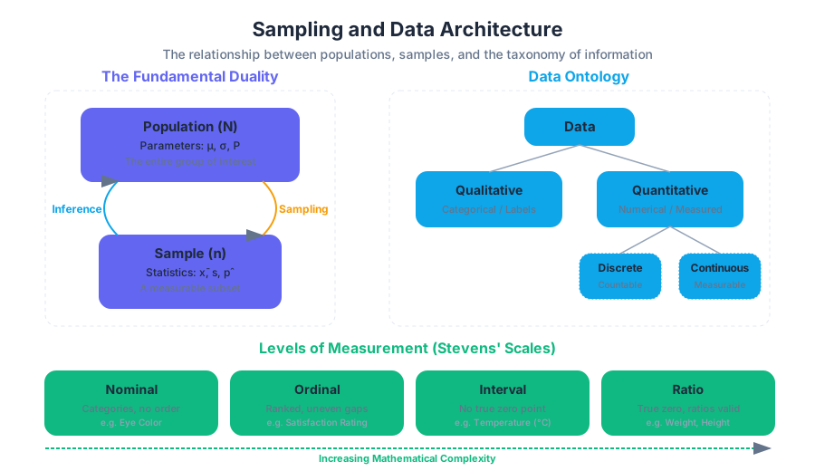
The Population is the complete collection of all individuals, objects, or measurements whose properties are being studied. It is the "universe" of our investigation. In mathematical notation, the size of a finite population is often denoted by $N$.
Definition: A Population is the entire group that is the target of an investigation. It is the set of all possible observations of a specific phenomenon.
The Sample
In practice, measuring every member of a population is often impossible due to constraints of time, cost, or accessibility. Instead, we select a Sample—a subset of the population. The size of a sample is denoted by $n$. The goal of sampling is to obtain a representative group that mirrors the characteristics of the population, allowing us to perform inferential statistics.
| Feature | Population | Sample |
|---|---|---|
| Definition | The entire group of interest. | A subset of the population. |
| Size Symbol | $N$ | $n$ |
| Accessibility | Often theoretical or inaccessible. | Tangible and measurable. |
| Goal | To understand the "true" state. | To estimate the population state. |
| Cost | Prohibitively high for large groups. | Manageable and optimized. |
Parameters vs. Statistics
The distinction between population and sample necessitates a distinction in the values we calculate from them. We use different terminology and symbols to clarify whether we are describing the "truth" of the population or an "estimate" from the sample.
Parameters
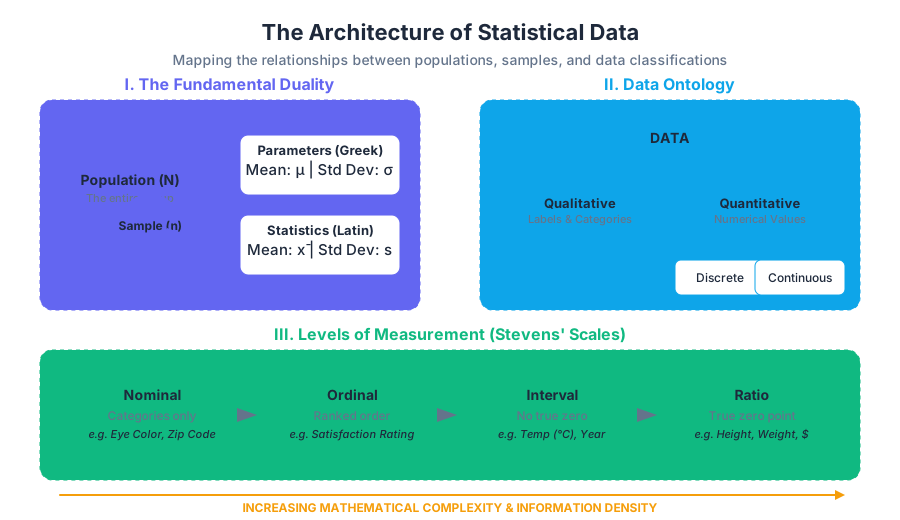
A Parameter is a numerical characteristic of a whole population. Because the population is usually not fully observed, parameters are often unknown constants. We represent parameters using Greek letters.
Statistics
A Statistic is a numerical characteristic of a sample. Unlike parameters, statistics are known once the data is collected. However, because samples vary, a statistic is a random variable. We represent statistics using Latin letters.
| Metric | Population Parameter (Greek) | Sample Statistic (Latin) |
|---|---|---|
| Mean (Average) | $\mu$ (mu) | $\bar{x}$ (x-bar) |
| Standard Deviation | $\sigma$ (sigma) | $s$ |
| Proportion | $P$ or $\pi$ (pi) | $\hat{p}$ (p-hat) |
| Variance | $\sigma^2$ | $s^2$ |
Key Insight: The central problem of statistics is Estimation. We use the sample statistic ($\bar{x}$) to make an educated guess about the population parameter ($\mu$). The difference between the two is known as the sampling error.
Data Ontology: Categorizing Information
Data is the raw material of statistics. To analyze it correctly, we must categorize it based on its mathematical properties. Not all data can be averaged, and not all data can be ranked.
Qualitative (Categorical) Data
Qualitative Data consists of attributes, labels, or non-numerical entries. These describe "qualities" rather than "quantities."
- Examples: Hair color, blood type, political affiliation, car make.
- Operations: We can count frequencies and calculate proportions, but we cannot calculate a "mean" hair color.
Quantitative (Numerical) Data
Quantitative Data consists of numbers that result from counting or measuring. These are further divided into two critical sub-types:
- Discrete Data: Data that can only take on specific, "countable" values. There are gaps between values.
- Example: The number of children in a family (you can't have 2.4 children).
- Continuous Data: Data that can take on any value within a range. It is usually the result of a measurement.
- Example: The weight of a person, the time spent waiting in line, the distance between cities.
| Data Type | Sub-type | Description | Example |
|---|---|---|---|
| Qualitative | N/A | Labels or categories. | Type of OS (Linux, Windows, macOS) |
| Quantitative | Discrete | Countable integers. | Number of CPU cores |
| Quantitative | Continuous | Measurable, infinite precision. | Processor clock speed (GHz) |
Levels of Measurement (Stevens' Scales)
Beyond the qualitative/quantitative split, we classify data into four levels of measurement. This hierarchy determines which statistical operations are mathematically valid.
- Nominal Level: Data that is classified into categories with no inherent order.
- Valid Ops: Mode, Frequency. (e.g., Zip codes, Gender).
- Ordinal Level: Data that can be ordered or ranked, but the differences between values are meaningless.
- Valid Ops: Median, Percentiles. (e.g., Movie ratings: 1-star, 2-star, 3-star).
- Interval Level: Data with a defined ordering and measurable differences, but no true zero point.
- Valid Ops: Addition, Subtraction, Mean. (e.g., Temperature in Celsius—0°C doesn't mean "no temperature").
- Ratio Level: Data with an ordering, measurable differences, and a true zero point (where zero means "none").
- Valid Ops: Multiplication, Division, Ratios. (e.g., Height, Weight, Salary).
Sampling Methodologies: The Mechanics of Collection
The validity of any statistical conclusion depends entirely on the quality of the sample. If a sample is not representative, it is biased, and the resulting statistics will systematically deviate from the true parameters.
1. Simple Random Sampling (SRS)
Every member of the population has an equal chance of being selected. This is the "gold standard" of sampling.
- Mechanism: Using a random number generator to pick $n$ individuals from a list of $N$.
2. Stratified Sampling
The population is divided into subgroups (strata) based on a specific characteristic (e.g., age, gender, income). A random sample is then taken from each stratum.
- Use Case: Ensuring that minority groups are adequately represented in the sample.
3. Cluster Sampling
The population is divided into groups (clusters), often geographically. A few clusters are selected at random, and all members within those selected clusters are sampled.
- Use Case: Large-scale surveys where it is too expensive to travel to every individual (e.g., sampling entire city blocks).
4. Systematic Sampling
Selecting every $k$-th individual from a list.
- Mechanism: Pick a random starting point between 1 and $k$, then select every $k$-th person thereafter.
5. Convenience Sampling
Selecting individuals who are easiest to reach.
- Warning: This method is highly prone to bias and is generally avoided in rigorous research.
| Method | Strategy | Best Used When... | Risk |
|---|---|---|---|
| Simple Random | Pure chance. | The population is homogeneous. | High variance in small samples. |
| Stratified | Sample from every group. | You want to compare subgroups. | Requires knowing strata in advance. |
| Cluster | Sample entire groups. | Population is spread out geographically. | Clusters may not represent the whole. |
| Systematic | Every $k$-th person. | You have a stream of data (e.g., assembly line). | Hidden patterns in the list order. |
Sampling in Practice
To understand how these concepts manifest in technical environments, we look at how data is sampled in code, mathematics, and database systems.
Mathematical Representation: The Logic of Inference
The relationship between a sample statistic and a population parameter is governed by the Sampling Distribution. For a sample mean $\bar{x}$, the expected value is the population mean $\mu$, but the precision depends on the sample size $n$.
\text{Let } X_1, X_2, \dots, X_n \text{ be i.i.d. random variables from a population with mean } \mu \text{ and variance } \sigma^2.

\text{The Sample Mean is defined as: }
\bar{x} = \frac{1}{n} \sum_{i=1}^{n} X_i

\text{The Expected Value of the Sample Mean is: }
E[\bar{x}] = E\left[\frac{1}{n} \sum X_i\right] = \frac{1}{n} \sum E[X_i] = \frac{1}{n} (n\mu) = \mu

\text{The Variance of the Sample Mean (Standard Error squared) is: }
Var(\bar{x}) = Var\left(\frac{1}{n} \sum X_i\right) = \frac{1}{n^2} \sum Var(X_i) = \frac{n\sigma^2}{n^2} = \frac{\sigma^2}{n}
Variation, Error, and Bias
Variation is natural; error is often structural. Understanding the difference is key to interpreting data.
Sampling Error
Even with a perfect random sampling method, the sample statistic will likely not equal the population parameter exactly. This discrepancy is Sampling Error. It is not a "mistake"—it is a natural consequence of using a subset to represent a whole. As $n$ increases, sampling error decreases.
Non-Sampling Error
These are errors caused by the data collection process itself. They do not disappear by increasing the sample size.
- Selection Bias: The sampling method systematically excludes certain segments of the population (e.g., an online survey excludes people without internet).
- Non-Response Bias: People who choose not to respond to a survey may have different opinions than those who do.
- Measurement Error: Poorly worded questions or faulty equipment lead to inaccurate data.
The Law of Large Numbers (LLN)
As the number of trials or the sample size increases, the sample mean $\bar{x}$ converges to the population mean $\mu$. This is the mathematical justification for why sampling works.
Common Pitfalls in Sampling
- Confusing "Random" with "Haphazard": Standing on a street corner and talking to whoever walks by is not random sampling; it is convenience sampling. A true random sample requires a sampling frame (a list) where every member has a known, non-zero probability of selection.
- Ignoring the "Small n" Problem: Small samples are highly susceptible to outliers. A single extreme value in a sample of 5 can swing the mean significantly, whereas it would be dampened in a sample of 500.
- Self-Selection Bias: Allowing subjects to volunteer for a study (e.g., Yelp reviews) creates a sample of people with strong opinions, which rarely represents the "average" experience.
- Treating Ordinal Data as Interval: Calculating the "average" of a Likert scale (1=Strongly Disagree, 5=Strongly Agree) is common but technically controversial, as the "distance" between "Neutral" and "Agree" may not be the same as the distance between "Agree" and "Strongly Agree."
Source Materials
Study Introductory Statistics on Lykke
This course page is free to open: signed out, you can read its first two sections, and signing in, on any plan, opens the rest. The free Lykke Chrome extension syncs your own Canvas courses, so ChatGPT, Claude and Muse can answer from your classes and deadlines. It only reads Canvas.
Add the free extensionSign in to open every sectionAll sections of Introductory Statistics · Browse more course pages