From the free course Introductory Statistics on Lykke
Linear Regression and Correlation
Key concepts: Correlation Coefficient (r) · Least-Squares Regression Line · Coefficient of Determination (r^2) · Residuals
Modeling the relationship between two quantitative variables and predicting outcomes.
Linear Regression and Correlation
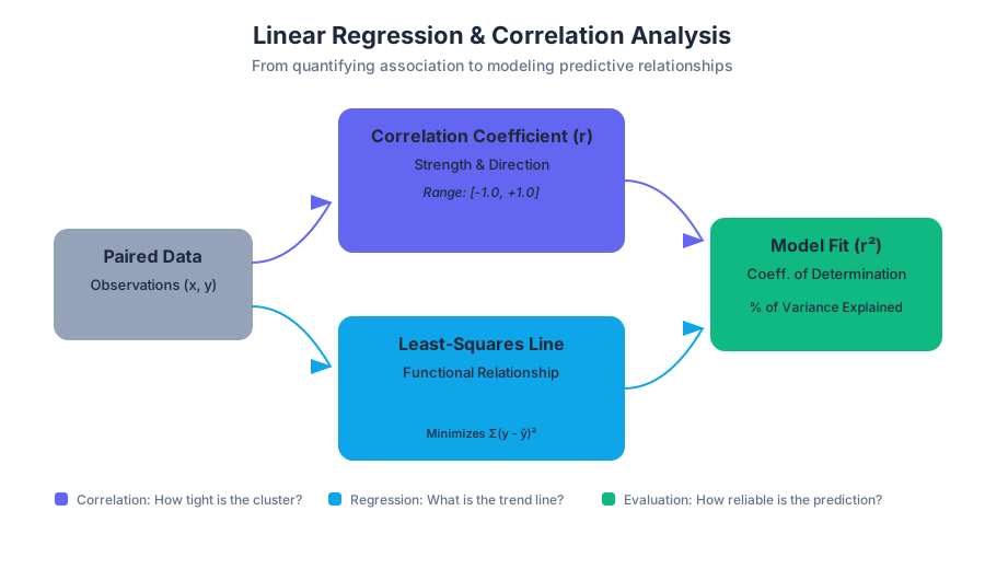
In the landscape of statistical modeling, the relationship between two quantitative variables serves as the bedrock for predictive analytics. Linear Regression and Correlation are the primary tools used to quantify the strength of these relationships and model the functional form they take. While correlation measures the degree of association, regression provides a mathematical framework to predict an outcome variable ($Y$) based on a predictor variable ($X$).
This article explores the mechanics of the Least-Squares Regression Line, the nuances of the Correlation Coefficient ($r$), the diagnostic power of Residuals, and the interpretative depth of the Coefficient of Determination ($r^2$).
The Correlation Coefficient ($r$)
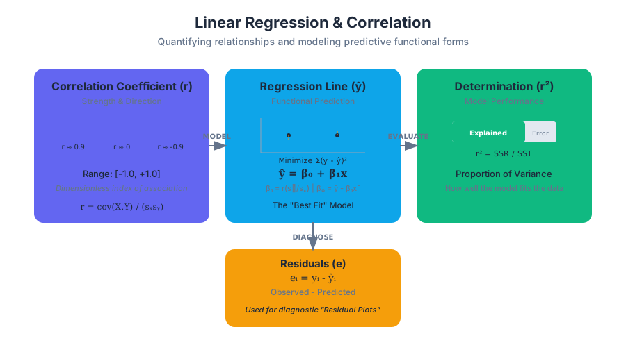
The Pearson Product-Moment Correlation Coefficient, denoted as $r$, is a dimensionless index that quantifies the linear relationship between two variables. Developed by Karl Pearson, it measures both the direction (positive or negative) and the strength (magnitude) of the linear association.
What it is
Mathematically, $r$ is the ratio of the covariance of the two variables to the product of their standard deviations. This normalization ensures that $r$ always falls within the range of $[-1, 1]$.
Definition: Pearson's $r$ For a sample of $n$ paired observations $(x_i, y_i)$, the correlation coefficient is defined as: $$r = \frac{\sum_{i=1}^{n} (x_i - \bar{x})(y_i - \bar{y})}{\sqrt{\sum_{i=1}^{n} (x_i - \bar{x})^2 \sum_{i=1}^{n} (y_i - \bar{y})^2}}$$
Why it matters
Correlation allows researchers to determine if a relationship exists before attempting to build a predictive model. It is the first step in exploratory data analysis (EDA). However, it is vital to remember that correlation does not imply causation; it merely indicates that the variables move together in a linear fashion.
Interpretation of $r$ Values
The magnitude of $r$ dictates the "tightness" of the data points around a central line.
| Value of $r$ | Interpretation | Visual Characteristic |
|---|---|---|
| $r = 1$ | Perfect Positive Correlation | All points lie exactly on a line with a positive slope. |
| $0.7 \le r < 1$ | Strong Positive | Points are closely clustered around an upward-sloping line. |
| $0.3 \le r < 0.7$ | Moderate Positive | A clear upward trend, but with significant dispersion. |
| $-0.3 < r < 0.3$ | Weak or No Correlation | Points appear as a "cloud" with no discernible linear trend. |
| $r = -1$ | Perfect Negative Correlation | All points lie exactly on a line with a negative slope. |
Least-Squares Regression Line
While correlation tells us how well two variables relate, Linear Regression tells us how they relate. It defines the functional relationship as a straight line: $\hat{y} = a + bx$ (or $\hat{y} = \beta_0 + \beta_1 x$ in formal notation).
The Principle of Least Squares
The "best-fit" line is defined as the line that minimizes the Sum of Squared Errors (SSE). An error (or residual) is the vertical distance between an observed data point and the predicted point on the line. By squaring these distances, we ensure that positive and negative errors don't cancel out and that larger errors are penalized more heavily.
The Objective Function Minimize $SSE = \sum (y_i - \hat{y}_i)^2 = \sum (y_i - (a + bx_i))^2$
Deriving the Coefficients
The slope ($b$) and the intercept ($a$) are derived using calculus (setting partial derivatives to zero) or via the following standard formulas:
b = \frac{\sum (x_i - \bar{x})(y_i - \bar{y})}{\sum (x_i - \bar{x})^2} = r \left( \frac{s_y}{s_x} \right)
a = \bar{y} - b\bar{x}
Mathematical Representation: The Normal Equations
In matrix form, the solution for the coefficients $\beta$ is found by solving the "Normal Equations." This is the foundation for all modern linear modeling software.
Given the model: Y = Xβ + ε
The goal is to solve for β that minimizes ||Y - Xβ||²

The solution is:
β = (XᵀX)⁻¹ XᵀY

Where:
- X is the design matrix (with a column of 1s for the intercept)
- Xᵀ is the transpose of X
- (XᵀX)⁻¹ is the inverse of the product of X transpose and X
- Y is the vector of observed values
Coefficient of Determination ($r^2$)
The Coefficient of Determination, denoted as $r^2$, is perhaps the most vital metric for evaluating the performance of a regression model. It represents the proportion of the variance in the dependent variable that is predictable from the independent variable.
Partitioning Variance
To understand $r^2$, we must view the total variation in $Y$ as being composed of two parts: the variation explained by the model and the variation left over (unexplained).
| Component | Symbol | Formula | Description |
|---|---|---|---|
| Total Sum of Squares | $SST$ | $\sum (y_i - \bar{y})^2$ | Total variation in the observed data. |
| Regression Sum of Squares | $SSR$ | $\sum (\hat{y}_i - \bar{y})^2$ | Variation explained by the linear relationship. |
| Error Sum of Squares | $SSE$ | $\sum (y_i - \hat{y}_i)^2$ | Unexplained variation (residuals). |
The relationship between these is: $SST = SSR + SSE$. Therefore, $r^2$ is defined as: $$r^2 = \frac{SSR}{SST} = 1 - \frac{SSE}{SST}$$
Interpretation
If $r^2 = 0.85$, we say that 85% of the variation in $Y$ is explained by the linear relationship with $X$. The remaining 15% is attributed to other factors or inherent random noise.
Residual Analysis
A model is only as good as its assumptions. Residuals ($e_i = y_i - \hat{y}_i$) are the "leftovers" of the model. Analyzing residuals is the primary way we diagnose whether a linear model is appropriate for the data.
The LINE Assumptions
For a linear regression model to be valid for inference, four conditions must be met:
- Linearity: The relationship between $X$ and $Y$ is linear.
- Independence: Observations are independent of each other.
- Normality: The residuals are normally distributed.
- Equal Variance (Homoscedasticity): The variance of residuals is constant across all levels of $X$.
Diagnostic Plots
A Residual Plot (Residuals vs. $X$ or $\hat{y}$) should ideally look like a random "snowstorm" of points centered around zero.
- Curved Pattern: Suggests the relationship is non-linear (e.g., quadratic).
- Fan Shape (Heteroscedasticity): Suggests the error variance changes as $X$ increases, violating the equal variance assumption.
- Outliers: Points with large residuals that may disproportionately pull the regression line.
Variations and Extensions
While simple linear regression involves one $X$ and one $Y$, the concept extends into several complex domains.
1. Multiple Linear Regression (MLR)
Predicting $Y$ using multiple independent variables: $\hat{y} = \beta_0 + \beta_1 x_1 + \beta_2 x_2 + ... + \beta_n x_n$. This allows for controlling confounding variables.
2. Non-linear Transformation
If the relationship is not linear, we can transform $X$ or $Y$ (e.g., $\log(x)$, $\sqrt{x}$, or $x^2$) to linearize the relationship before fitting the model.
3. Influential Points and Leverage
Not all data points are created equal.
- Outliers: Observations with extreme $Y$ values.
- High Leverage Points: Observations with extreme $X$ values.
- Influential Points: A point that, if removed, significantly changes the slope or intercept of the regression line.
| Metric | Purpose | Threshold Idea |
|---|---|---|
| Cook's Distance | Measures influence of a single point. | Values > 1 often indicate high influence. |
| Standard Error ($s_e$) | Measures the average distance points fall from the line. | Smaller is better; used for confidence intervals. |
| p-value for Slope | Tests $H_0: \beta_1 = 0$. | If $p < 0.05$, the relationship is statistically significant. |
Common Pitfalls and Misconceptions
1. Extrapolation
Predicting $Y$ values for $X$ values outside the range of the original data is dangerous. We have no evidence that the linear relationship continues indefinitely. For example, a model relating height to age in children cannot be extrapolated to predict the height of a 60-year-old.
2. Correlation $\neq$ Causation
A high $r$ value between "Ice Cream Sales" and "Drowning Incidents" does not mean ice cream causes drowning. Both are driven by a lurking variable: warm weather.
3. The Influence of Outliers
A single extreme outlier can inflate or deflate $r$ and significantly tilt the regression line, leading to a model that represents the outlier better than the bulk of the data.
4. Interpreting $r^2$ as Accuracy
$r^2$ measures "explained variance," not necessarily "accuracy." A model can have a high $r^2$ but still produce large prediction errors if the underlying variance of the data is high.
Practical Example: Real Estate Valuation
Imagine a dataset where $X$ is the square footage of a house and $Y$ is the sale price.
- Correlation: We find $r = 0.92$, indicating a very strong positive relationship.
- Regression: The line is $\hat{y} = 50,000 + 150x$.
- The Intercept ($50,000$) suggests the base price of a lot before building.
- The Slope ($150$) means for every additional square foot, the price increases by $\text{\textdollar}150$.
- Coefficient of Determination: $r^2 = 0.846$. This means 84.6% of the price variation is explained by size. The other 15.4% might be due to location, age, or interior finishes.
- Residuals: A house that sold for $\text{\textdollar}300,000$ but was predicted at $\text{\textdollar}280,000$ has a residual of $+\text{\textdollar}20,000$. This house was "overpriced" or had premium features not captured by square footage alone.
Source Materials
Study Introductory Statistics on Lykke
This course page is free to open: signed out, you can read its first two sections, and signing in, on any plan, opens the rest. The free Lykke Chrome extension syncs your own Canvas courses, so ChatGPT, Claude and Muse can answer from your classes and deadlines. It only reads Canvas.
Add the free extensionSign in to open every sectionAll sections of Introductory Statistics · Browse more course pages