From the free course Introductory Statistics on Lykke
Hypothesis Testing with Two Samples
Key concepts: Independent Samples · Matched Pairs · Difference of Means · Pooled Variance
Comparing two different populations to see if there is a significant difference between them.
Hypothesis Testing with Two Samples
In the landscape of statistical inference, single-sample testing serves as a foundational proof of concept. However, empirical science rarely operates in a vacuum. The most critical questions in medicine, engineering, and social science are comparative: Does Drug A outperform Drug B? Does a new manufacturing process reduce defects compared to the legacy system? Do two demographic groups exhibit different behavioral patterns?
Hypothesis testing with two samples allows us to determine if the observed differences between two groups are statistically significant or merely the result of stochastic noise. This requires a sophisticated understanding of how variances interact, how samples are related, and how the geometry of the sampling distribution changes when we move from a single point estimate to a difference of estimates.
The Taxonomy of Two-Sample Tests
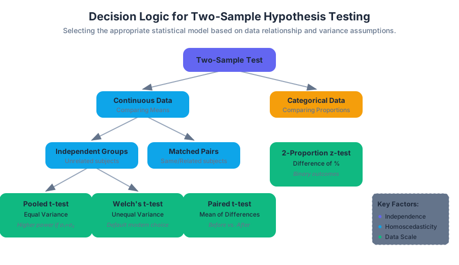
Before selecting a mathematical model, a researcher must identify the relationship between the two samples and the nature of the data. The choice of test is governed by three primary factors: the independence of the groups, the equality of their variances, and the type of data (means vs. proportions).
| Test Type | Data Requirement | Relationship | Key Statistic |
|---|---|---|---|
| Independent t-test (Welch’s) | Continuous | Unrelated groups | Difference of means, unequal variance |
| Pooled Variance t-test | Continuous | Unrelated groups | Difference of means, equal variance |
| Paired/Matched t-test | Continuous | Related/Same subjects | Mean of differences |
| Two-Proportion z-test | Categorical/Binary | Unrelated groups | Difference of proportions |
Independent Samples: Comparing Unrelated Means
Independent samples occur when the subjects in one group provide no information about the subjects in the second group. For example, testing the blood pressure of a group in New York versus a group in Tokyo.
The Aspin-Welch T-Test (Unequal Variance)
In modern computational statistics, the Aspin-Welch t-test is the default choice. Unlike the classical Student’s t-test, it does not assume that the two populations have the same variance (homoscedasticity).
Definition: The Welch’s t-test is an adaptation of the Student's t-test used to compare two samples with potentially unequal variances and unequal sample sizes. It utilizes a modified calculation for the degrees of freedom ($df$) known as the Welch-Satterthwaite equation.
The test statistic is calculated as: $$t = \frac{(\bar{x}_1 - \bar{x}_2) - (\mu_1 - \mu_2)}{\sqrt{\frac{s_1^2}{n_1} + \frac{s_2^2}{n_2}}}$$
Where:
- $\bar{x}_1, \bar{x}_2$: Sample means
- $s_1, s_2$: Sample standard deviations
- $n_1, n_2$: Sample sizes
The complexity arises in the Degrees of Freedom, which is no longer a simple integer ($n-1$): $$df = \frac{(\frac{s_1^2}{n_1} + \frac{s_2^2}{n_2})^2}{\frac{(s_1^2/n_1)^2}{n_1-1} + \frac{(s_2^2/n_2)^2}{n_2-1}}$$
The Case for Pooled Variance
While Welch's t-test is robust, the Pooled Variance t-test is used when we have a strong theoretical reason to believe the population variances are equal ($\sigma_1^2 = \sigma_2^2$). This often occurs in controlled laboratory settings where the same equipment and processes are used on different subjects.
Mechanics of Pooling
By "pooling" the variance, we create a weighted average of the two sample variances, which provides a more precise estimate of the common population variance.
Theorem (Pooled Variance): If $\sigma_1 = \sigma_2$, the best estimate of the common variance $s_p^2$ is: $$s_p^2 = \frac{(n_1 - 1)s_1^2 + (n_2 - 1)s_2^2}{n_1 + n_2 - 2}$$
The standard error then becomes $SE = \sqrt{s_p^2 (\frac{1}{n_1} + \frac{1}{n_2})}$. The degrees of freedom for this test is simply $n_1 + n_2 - 2$.
Comparison of Variance Strategies
| Strategy | Assumption | Risk | Benefit |
|---|---|---|---|
| Welch's (Default) | $\sigma_1 \neq \sigma_2$ | Slightly lower power if variances are actually equal. | Robust against Type I errors when variances differ. |
| Pooled | $\sigma_1 = \sigma_2$ | High Type I error rate if variances are unequal (especially with unequal $n$). | Higher statistical power if the assumption holds. |
Matched or Paired Samples: The Dependent Case
In a Matched Pairs design (also called Dependent Samples), the two sets of data are intrinsically linked. This is most common in "Before and After" studies or "Twin Studies."
The Logic of Difference
Instead of comparing two separate distributions, we transform the problem into a single-sample test. We calculate the difference ($d$) for each pair: $$d_i = x_{1,i} - x_{2,i}$$
We then test the null hypothesis that the mean of these differences is zero ($H_0: \mu_d = 0$).
Mathematical Derivation of the Paired T-Statistic
Given pairs (X_i, Y_i) for i = 1 to n:
1. Calculate d_i = X_i - Y_i
2. Calculate the sample mean of differences:
   d_bar = (1/n) * Σ d_i
3. Calculate the sample standard deviation of differences:
   s_d = sqrt( [Σ (d_i - d_bar)^2] / (n - 1) )
4. Calculate the standard error:
   SE = s_d / sqrt(n)
5. The t-statistic follows:
   t = (d_bar - μ_d) / SE
   where μ_d is typically 0 under H0.
6. Degrees of Freedom:
   df = n - 1 (where n is the number of pairs)
Why Use Paired Samples?
Pairing is a powerful tool for noise reduction. By using the same subject for both measurements, we control for "inter-subject variability." If a drug lowers blood pressure by 5 points, it might be hard to see that in two independent groups because individual blood pressures vary by 50 points. But in a paired test, that 5-point drop is visible for every single person, regardless of their starting baseline.
Comparing Two Proportions
When the outcome is binary (Success/Failure, Yes/No), we compare proportions ($p_1$ and $p_2$). This is the standard for A/B testing in software engineering and clinical trials.
The Pooled Proportion
Under the null hypothesis $H_0: p_1 = p_2$, we assume both samples come from a population with a single, common proportion. We estimate this by pooling the successes:
$$\hat{p}_c = \frac{x_1 + x_2}{n_1 + n_2}$$
Where $x_1$ and $x_2$ are the number of successes in each group.
The Z-Statistic for Proportions
The test statistic follows a standard normal distribution: $$z = \frac{(\hat{p}_1 - \hat{p}_2) - 0}{\sqrt{\hat{p}_c(1-\hat{p}_c)(\frac{1}{n_1} + \frac{1}{n_2})}}$$
Effect Size: Cohen’s d
A common pitfall in two-sample testing is confusing statistical significance with practical significance. With a large enough sample size ($n > 10,000$), even a tiny, meaningless difference will yield a $p < 0.05$.
To measure the magnitude of the difference, we use Cohen's d.
Definition: Cohen's d measures the distance between two means in units of standard deviation.
$$d = \frac{\bar{x}_1 - \bar{x}2}{s{pooled}}$$
| Cohen's d | Effect Size | Interpretation |
|---|---|---|
| 0.2 | Small | Difference is hard to see with the naked eye. |
| 0.5 | Medium | Difference is visible to a trained observer. |
| 0.8 | Large | Difference is obvious; distributions have minimal overlap. |
Common Pitfalls and Assumptions
1. The Normality Assumption
Both the t-test and the z-test assume that the underlying populations are normally distributed. However, due to the Central Limit Theorem, these tests are remarkably robust for large sample sizes ($n_1, n_2 > 30$), even if the data is skewed.
2. Data Snooping (P-Hacking)
Testing multiple pairs of groups until one shows a significant result is a violation of statistical ethics. If you compare 20 different groups, one will likely show a significant difference by pure chance ($0.05 \times 20 = 1$).
3. Ignoring Outliers
Two-sample tests are sensitive to outliers, especially in small samples. A single extreme value can inflate the variance, blowing up the denominator of the t-statistic and making a truly significant difference appear insignificant.
4. Confusing Independent and Paired Designs
Using an independent t-test on paired data is a "conservative error"—it will likely fail to find a significant difference that actually exists because it ignores the correlation between the pairs, resulting in an inflated standard error.
Summary of Workflow
- Identify the Goal: Are you comparing means or proportions?
- Check Independence: Are the groups unrelated or paired?
- Verify Assumptions: Check for normality and outliers.
- Choose the Variance Strategy: Default to Welch’s unless equal variance is strictly guaranteed.
- Calculate the Statistic: Compute $t$ or $z$ and the corresponding $p$-value.
- Evaluate Effect Size: Calculate Cohen’s $d$ to determine if the result matters in the real world.
- Conclude: Reject or fail to reject $H_0$ based on the alpha level (typically 0.05).

Source Materials
Study Introductory Statistics on Lykke
This course page is free to open: signed out, you can read its first two sections, and signing in, on any plan, opens the rest. The free Lykke Chrome extension syncs your own Canvas courses, so ChatGPT, Claude and Muse can answer from your classes and deadlines. It only reads Canvas.
Add the free extensionSign in to open every sectionAll sections of Introductory Statistics · Browse more course pages