From the free course Introductory Statistics on Lykke
Hypothesis Testing with One Sample
Key concepts: Null Hypothesis (H0) · Alternative Hypothesis (Ha) · P-value · Significance Level (Alpha) · Type I and II Errors
The formal process for testing claims about a population using a single sample.
Hypothesis Testing with One Sample
Hypothesis testing is the formal statistical backbone of the scientific method. It provides a rigorous framework for moving beyond mere observation into the realm of inferential statistics, where we use sample data to make probabilistic statements about an entire population. At its core, hypothesis testing is a "proof by contradiction" mechanism: we assume a default state of the world (the Null Hypothesis) and determine if our observed data is so unlikely under that assumption that we are forced to reject it in favor of a new explanation.
In a one-sample context, we are typically comparing a single sample mean ($\bar{x}$) or proportion ($\hat{p}$) against a known or hypothesized population parameter ($\mu_0$ or $p_0$). This process is essential in quality control, medical research, and A/B testing, where one must decide if a deviation from the norm is a genuine effect or simply the result of stochastic noise.
The Logical Framework: $H_0$ and $H_a$
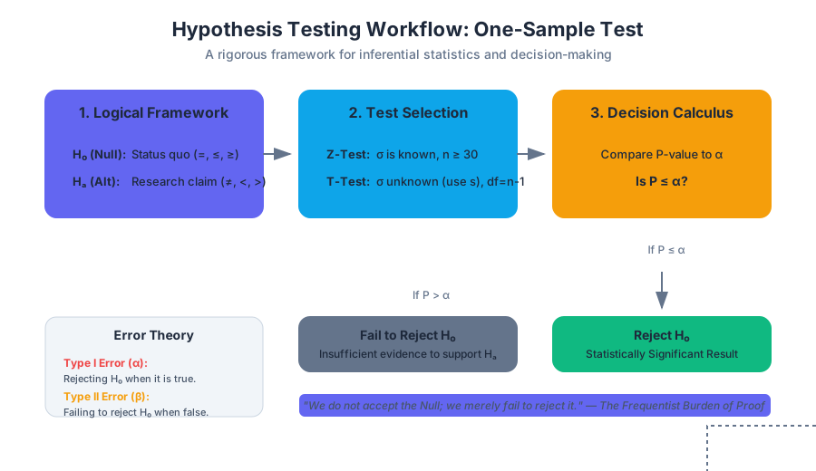
The foundation of any test lies in the construction of two mutually exclusive and collectively exhaustive statements.
The Null Hypothesis ($H_0$)
The Null Hypothesis represents the status quo, the "no-effect" state, or the assumption that any observed difference is due to chance. In a one-sample test, $H_0$ always contains an equality ($=, \le, \text{ or } \ge$).
The Alternative Hypothesis ($H_a$)
The Alternative Hypothesis (sometimes denoted as $H_1$) is the claim the researcher hopes to support. It represents a departure from the status quo. $H_a$ never contains an equality ($<, >, \text{ or } \neq$).
| Hypothesis Type | Notation | Logical Role | Mathematical Symbols |
|---|---|---|---|
| Null | $H_0$ | The "Innocent" plea; the baseline assumption. | $=, \leq, \geq$ |
| Alternative | $H_a$ | The "Guilty" verdict; the research claim. | $\neq, >, <$ |
The Burden of Proof: In the Frequentist tradition, the burden of proof lies entirely on the Alternative Hypothesis. We do not "accept" the Null; we merely "fail to reject" it if the evidence is insufficient. This is analogous to a court of law where a defendant is found "not guilty" rather than "innocent."
The Decision Calculus: P-values and Alpha ($\alpha$)
To decide between $H_0$ and $H_a$, we need a threshold for "unlikeliness."
Significance Level ($\alpha$)
The Significance Level ($\alpha$) is the probability threshold set by the researcher before the experiment. It defines the maximum risk of rejecting a true null hypothesis that the researcher is willing to take. Common values include 0.05, 0.01, and 0.10.
The P-value
The P-value is the probability of obtaining a test statistic at least as extreme as the one observed, assuming the null hypothesis is true. It is NOT the probability that the null hypothesis is true; rather, it is $P(\text{Data} | H_0)$.
Decision Rules
- If P-value $\le \alpha$: The result is statistically significant. Reject $H_0$.
- If P-value $> \alpha$: The result is not statistically significant. Fail to reject $H_0$.
Statistical Error Theory: Type I and Type II
Because we are working with samples rather than entire populations, our decisions are subject to two types of errors.
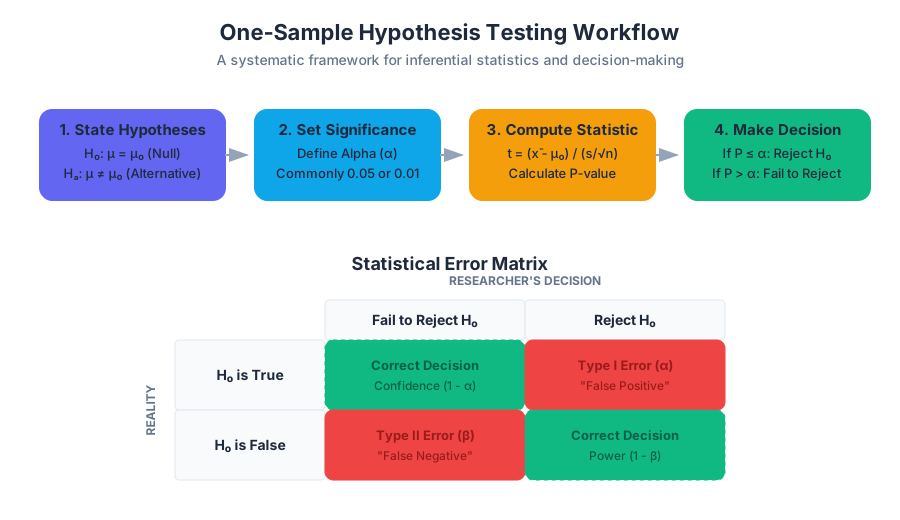
- Type I Error ($\alpha$): Rejecting $H_0$ when it is actually true (a "False Positive").
- Type II Error ($\beta$): Failing to reject $H_0$ when it is actually false (a "False Negative").
| Reality \ Decision | Fail to Reject $H_0$ | Reject $H_0$ |
|---|---|---|
| $H_0$ is True | Correct Decision (Confidence: $1-\alpha$) | Type I Error (Significance: $\alpha$) |
| $H_0$ is False | Type II Error ($\beta$) | Correct Decision (Power: $1-\beta$) |
The Power of a Test
The Power of a statistical test ($1 - \beta$) is the probability that the test will correctly reject a false null hypothesis. Increasing the sample size ($n$) or the effect size generally increases the power of the test.
Mechanics of the One-Sample Test
The choice of test depends on whether the population standard deviation ($\sigma$) is known and whether the sample size is large enough for the Central Limit Theorem to apply.
1. The One-Sample Z-Test
Used when the population variance $\sigma^2$ is known and the population is normally distributed or the sample size $n$ is large ($n \ge 30$).
2. The One-Sample T-Test
Used when the population variance $\sigma^2$ is unknown (which is almost always the case in practice). It uses the sample standard deviation ($s$) and follows the Student's t-distribution with $n-1$ degrees of freedom ($df$).
Mathematical Derivation (LaTeX/Math)
The following represents the formal derivation of the test statistic and the probability density function for the T-distribution.
\text{The Test Statistic for a One-Sample T-Test is defined as:}
\\
t = \frac{\bar{x} - \mu_0}{s / \sqrt{n}}
\\
\text{Where:}
\begin{cases}
\bar{x} & \text{Sample Mean} \\
\mu_0 & \text{Hypothesized Population Mean} \\
s & \text{Sample Standard Deviation} \\
n & \text{Sample Size}
\end{cases}
\\
\text{The Probability Density Function (PDF) of the T-distribution with } \nu \text{ degrees of freedom:}
\\
f(t) = \frac{\Gamma(\frac{\nu+1}{2})}{\sqrt{\nu\pi}\,\Gamma(\frac{\nu}{2})} \left(1+\frac{t^2}{\nu}\right)^{-\frac{\nu+1}{2}}
Step-by-Step Execution of a One-Sample Test
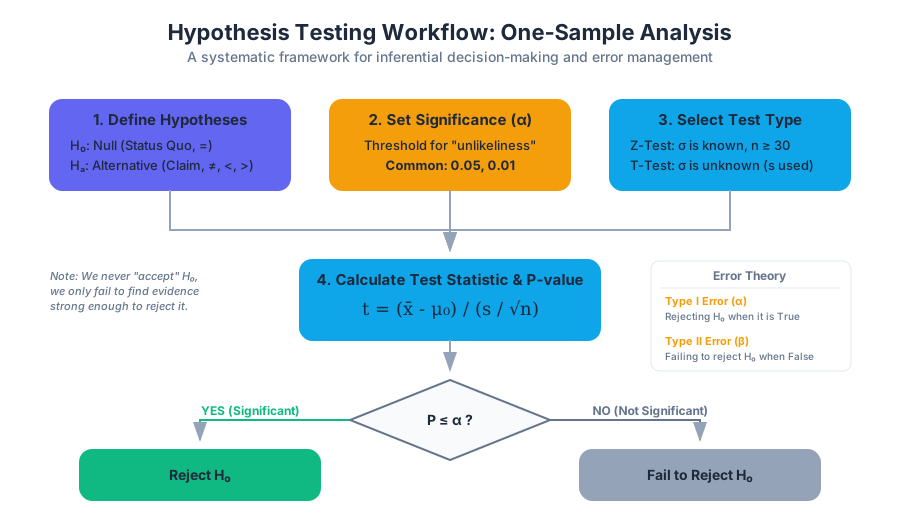
To ensure scientific validity, a hypothesis test must follow a standardized pipeline.
Step 1: State the Hypotheses
Define $H_0$ and $H_a$ clearly. Determine if the test is one-tailed (directional, e.g., "greater than") or two-tailed (non-directional, e.g., "different from").
Step 2: Set the Criteria
Choose the significance level $\alpha$. In high-stakes fields like pharmaceuticals, $\alpha$ might be 0.01; in social sciences, 0.05 is standard.
Step 3: Verify Assumptions
- Independence: Observations must be independent of each other.
- Randomness: Data should be collected via a random sampling method.
- Normality: The population should be normally distributed, or $n$ should be large enough (Central Limit Theorem).
Step 4: Calculate the Test Statistic and P-value
Compute the Z or T score and find the corresponding P-value using distribution tables or software.
Step 5: Make the Decision
Compare the P-value to $\alpha$ and state the conclusion in the context of the original problem.
| Component | Two-Tailed Test | One-Tailed Test (Right) | One-Tailed Test (Left) |
|---|---|---|---|
| $H_a$ | $\mu \neq \mu_0$ | $\mu > \mu_0$ | $\mu < \mu_0$ |
| Rejection Region | Both tails | Right tail | Left tail |
| P-value Calc | $2 \times P(T > | t | )$ |
Critical Extensions: Effect Size and Confidence Intervals
A common pitfall in hypothesis testing is over-reliance on the P-value. With a large enough sample size, even a trivial difference can become "statistically significant." To counter this, we use Effect Size.
Cohen's $d$
Cohen's $d$ measures the magnitude of the difference in terms of standard deviations. $$d = \frac{|\bar{x} - \mu_0|}{s}$$
| Effect Size | Cohen's $d$ Value |
|---|---|
| Small | 0.2 |
| Medium | 0.5 |
| Large | 0.8 |
Confidence Intervals (CI)
A Confidence Interval provides a range of plausible values for the population parameter. If the hypothesized mean $\mu_0$ falls outside the $(1-\alpha)$ confidence interval, we reject $H_0$ at the $\alpha$ level.
Common Pitfalls and Misconceptions
- "P-hacking": Running multiple tests or adjusting the sample size until a significant P-value is found. This inflates the Type I error rate.
- Misinterpreting the P-value: Thinking a P-value of 0.05 means there is a 95% chance the alternative hypothesis is true.
- Absence of Evidence vs. Evidence of Absence: Failing to reject $H_0$ does not prove $H_0$ is true; it simply means the data is not strong enough to prove otherwise.
- Statistical vs. Practical Significance: A result can be statistically significant ($p < 0.05$) but practically useless if the effect size is near zero.
Summary of the Decision Matrix
When approaching a one-sample problem, use this logic flow:
- Is the data continuous? (If yes, proceed to Means. If no, use Proportions).
- Is $\sigma$ known? (If yes, use Z-test. If no, use T-test).
- Is $n < 30$? (If yes, the population must be normal to use the T-test).
- Is the claim directional? (If yes, use a one-tailed test).
Source Materials
Study Introductory Statistics on Lykke
This course page is free to open: signed out, you can read its first two sections, and signing in, on any plan, opens the rest. The free Lykke Chrome extension syncs your own Canvas courses, so ChatGPT, Claude and Muse can answer from your classes and deadlines. It only reads Canvas.
Add the free extensionSign in to open every sectionAll sections of Introductory Statistics · Browse more course pages