From the free course Introductory Statistics on Lykke
Descriptive Statistics
Key concepts: Mean · Median · Mode · Standard Deviation · Box Plots · Histograms
Methods for summarizing and visualizing data sets using graphical representations and numerical measures.
Descriptive Statistics
Descriptive statistics represents the foundational layer of data science and analytical reasoning. Rather than making inferences about a population from a sample, descriptive statistics focuses on the characterization and summarization of the data currently at hand. It is the process of data compression: taking a raw dataset—which may contain millions of individual observations—and distilling it into a few interpretable values and visualizations that capture its essence.
In the modern data pipeline, descriptive statistics serves as the "Sanity Check" phase. Before complex machine learning models are deployed or hypothesis tests are conducted, an analyst must understand the central tendency, the dispersion, and the shape of the data distribution. Without this, one risks the "Garbage In, Garbage Out" (GIGO) failure mode, where outliers or skewed distributions invalidate downstream logic.
Measures of Central Tendency
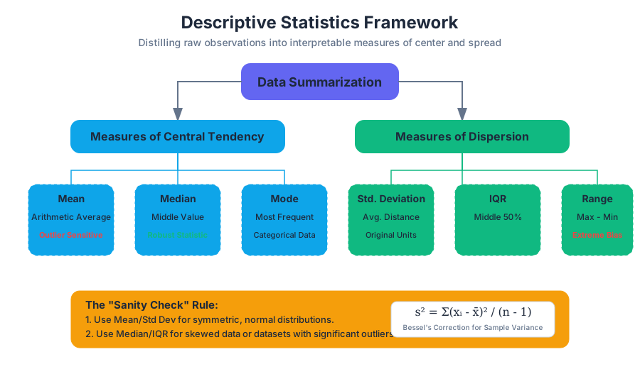
Central tendency refers to the "typical" or "middle" value of a dataset. While the concept seems intuitive, the choice of which measure to use depends heavily on the data's scale, distribution, and the presence of outliers.
The Mean (Arithmetic Average)
The Mean is the sum of all values divided by the number of observations. Mathematically, for a sample $x$, it is denoted as $\bar{x}$:
Definition: Arithmetic Mean $$\bar{x} = \frac{1}{n} \sum_{i=1}^{n} x_i$$ Where $n$ is the number of observations and $x_i$ represents each individual value.
The mean is the "balance point" of the data. However, it is highly sensitive to outliers. A single extreme value can pull the mean far away from the bulk of the data, making it a poor representation of "typicality" in skewed datasets (e.g., household income).
The Median
The Median is the middle value when the data is sorted in ascending or descending order. If the dataset has an even number of observations, the median is the average of the two central values.
The median is a robust statistic. Unlike the mean, it is resistant to outliers. In a dataset of $[10, 20, 30, 40, 1000]$, the mean is $220$, while the median is $30$. The median provides a better sense of the "typical" value in this context.
The Mode
The Mode is the value that appears most frequently in a dataset. A distribution can be unimodal (one mode), bimodal (two modes), or multimodal. It is the only measure of central tendency that can be used with nominal (categorical) data, such as "favorite color" or "operating system."
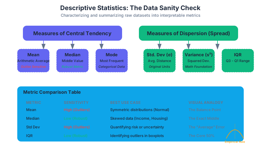
| Metric | Sensitivity to Outliers | Data Type Suitability | Best Use Case |
|---|---|---|---|
| Mean | High | Interval, Ratio | Symmetric distributions (e.g., heights) |
| Median | Low (Robust) | Ordinal, Interval, Ratio | Skewed distributions (e.g., salaries) |
| Mode | Low | Nominal, Ordinal, Discrete | Categorical data (e.g., most popular product) |
Measures of Dispersion (Spread)
Knowing the center of the data is insufficient. Two datasets can have the exact same mean but look entirely different. Dispersion describes how spread out the values are around the center.
Variance and Standard Deviation
The Variance ($\sigma^2$ for population, $s^2$ for sample) measures the average squared deviation from the mean. Because variance is in "squared units," we take its square root to get the Standard Deviation ($\sigma$ or $s$), which returns the measure to the original units of the data.
Theorem: Bessel's Correction When calculating the sample variance ($s^2$), we divide by $n-1$ instead of $n$. This corrects the bias in the estimation of the population variance, as a sample tends to underestimate the true spread of the population. $$s^2 = \frac{\sum (x_i - \bar{x})^2}{n - 1}$$
Range and Interquartile Range (IQR)
- Range: The difference between the maximum and minimum values. It is extremely sensitive to outliers.
- IQR: The difference between the 75th percentile ($Q_3$) and the 25th percentile ($Q_1$). It represents the spread of the middle 50% of the data and is a robust measure of dispersion.
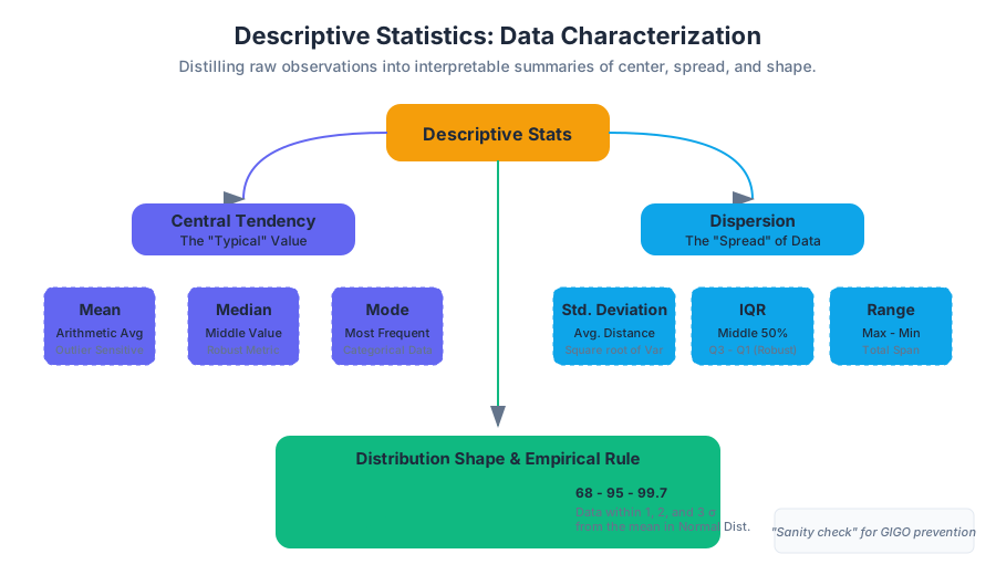
The Empirical Rule (68-95-99.7)
For data that follows a Normal Distribution (bell curve):
- Approximately 68% of the data falls within $1\sigma$ of the mean.
- Approximately 95% falls within $2\sigma$.
- Approximately 99.7% falls within $3\sigma$.
Mathematical Derivation: Variance
ALGORITHM CalculateSampleVariance(Dataset X):
    1.  n = length(X)
    2.  IF n < 2 THEN RETURN 0

    3.  Sum = 0
    4.  FOR EACH value x IN X:
            Sum = Sum + x
    5.  Mean = Sum / n

    6.  SumOfSquaredDeviations = 0
    7.  FOR EACH value x IN X:
            Deviation = x - Mean
            SquaredDeviation = Deviation * Deviation
            SumOfSquaredDeviations = SumOfSquaredDeviations + SquaredDeviation

    8.  Variance = SumOfSquaredDeviations / (n - 1)  // Applying Bessel's Correction
    9.  RETURN Variance
Graphical Displays: Visualizing the Distribution
Numerical summaries can be deceptive (see: Anscombe's Quartet). Visualization is essential to reveal the "shape" of the data.
Histograms
A Histogram groups continuous data into "bins" and displays the frequency of observations within each bin. It is the primary tool for identifying the shape of a distribution:
- Symmetric: The left and right sides are mirror images.
- Left-Skewed (Negative): The tail extends to the left; the mean is typically less than the median.
- Right-Skewed (Positive): The tail extends to the right; the mean is typically greater than the median.
Box Plots (Box-and-Whisker)
A Box Plot provides a visual summary of the "Five-Number Summary":
- Minimum: The lowest data point (excluding outliers).
- First Quartile ($Q_1$): The 25th percentile.
- Median ($Q_2$): The 50th percentile.
- Third Quartile ($Q_3$): The 75th percentile.
- Maximum: The highest data point (excluding outliers).
Outliers in a box plot are typically defined using Tukey’s Fences: any point more than $1.5 \times IQR$ above $Q_3$ or below $Q_1$.
| Feature | Histogram | Box Plot |
|---|---|---|
| Primary Goal | Show the shape/density of distribution. | Show quartiles, spread, and outliers. |
| Granularity | High (depends on bin size). | Low (summarizes into 5 points). |
| Outlier Detection | Visual gaps in bars. | Explicitly marked points. |
| Comparison | Hard to overlay many distributions. | Excellent for comparing multiple groups side-by-side. |
Advanced Concepts: Skewness and Kurtosis
Beyond center and spread, we describe the "style" of the distribution's shape.
Skewness
Skewness measures the asymmetry of the probability distribution.
- A skewness of 0 indicates perfect symmetry.
- Positive skew indicates a long right tail (common in wealth distribution).
- Negative skew indicates a long left tail (common in age of retirement).
Kurtosis
Kurtosis measures the "tailedness" of the distribution.
- Mesokurtic: Similar to a normal distribution (Kurtosis $\approx 3$).
- Leptokurtic: Heavy tails and a sharp peak (indicates frequent extreme outliers).
- Platykurtic: Thin tails and a flat peak (indicates fewer outliers than a normal distribution).
Common Pitfalls in Descriptive Statistics
- Over-reliance on the Mean: Using the mean for highly skewed data (like startup valuations) leads to a distorted view of reality. Always check the median.
- Binning Bias in Histograms: Choosing bins that are too wide hides patterns; choosing bins that are too narrow creates noise. Use the Freedman-Diaconis rule for optimal bin width: $h = 2 \frac{IQR(x)}{\sqrt[3]{n}}$.
- Ignoring the Sample Size: A standard deviation of 10 means something very different if $n=5$ versus $n=5000$.
- Confusing Standard Deviation with Standard Error: Standard deviation describes the spread of the data, while standard error describes the uncertainty of the mean estimate.
Practical Example: Analyzing Server Latency
Imagine you are a Site Reliability Engineer (SRE) monitoring API response times.
- Mean Latency: 200ms.
- Median Latency: 150ms.
- 99th Percentile (P99): 2500ms.
If you only looked at the mean, you might think the system is performing well. However, the gap between the median (150ms) and the mean (200ms) suggests a right-skewed distribution. The P99 of 2500ms reveals that while most users have a fast experience, 1% of users are experiencing a 2.5-second delay—a critical issue that the mean obscures.
Summary Table: Choosing the Right Statistic
| Scenario | Recommended Measure | Why? |
|---|---|---|
| Reporting average salaries | Median | Prevents high-earning outliers from inflating the "average." |
| Manufacturing quality control | Standard Deviation | Measures consistency; lower is better. |
| Analyzing website traffic spikes | Mode | Identifies the most common time of day users visit. |
| Comparing test scores across classes | Box Plot | Shows the spread and identifies struggling/excelling students easily. |
| Determining "normal" heart rate | Mean + Std Dev | Heart rate is generally normally distributed in healthy populations. |
Source Materials
Study Introductory Statistics on Lykke
This course page is free to open: signed out, you can read its first two sections, and signing in, on any plan, opens the rest. The free Lykke Chrome extension syncs your own Canvas courses, so ChatGPT, Claude and Muse can answer from your classes and deadlines. It only reads Canvas.
Add the free extensionSign in to open every sectionAll sections of Introductory Statistics · Browse more course pages