From the free course Introductory Statistics on Lykke
Continuous Random Variables
Key concepts: Uniform Distribution · Exponential Distribution · Density Curves · Area under the Curve
Introduction to variables that can take any value within a range, focusing on the Uniform and Exponential distributions.
Continuous Random Variables
In the study of probability and statistics, we distinguish between two fundamental types of data: discrete and continuous. While discrete random variables deal with "countable" outcomes—the number of heads in a coin toss or the number of students in a classroom—continuous random variables represent measurements on a continuum. These variables can take on any value within a given range, often involving decimals or fractions of infinite precision.
From the perspective of a data scientist or engineer, the shift from discrete to continuous is a shift from summation to integration. We no longer ask for the probability that a variable equals a specific value; instead, we measure the probability that a variable falls within a specific interval. This distinction is the bedrock of modern statistical modeling, from predicting the lifespan of server hardware to modeling the latency of a microservice.
The Geometry of Probability: Density Curves
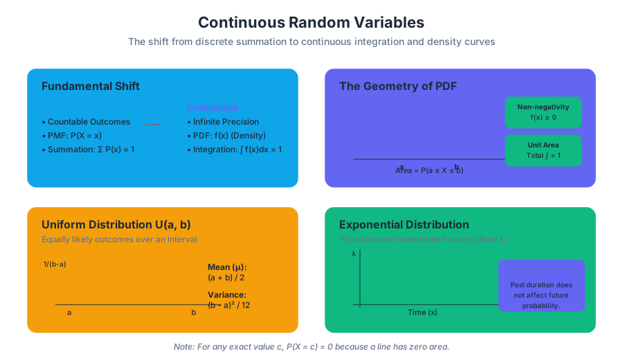
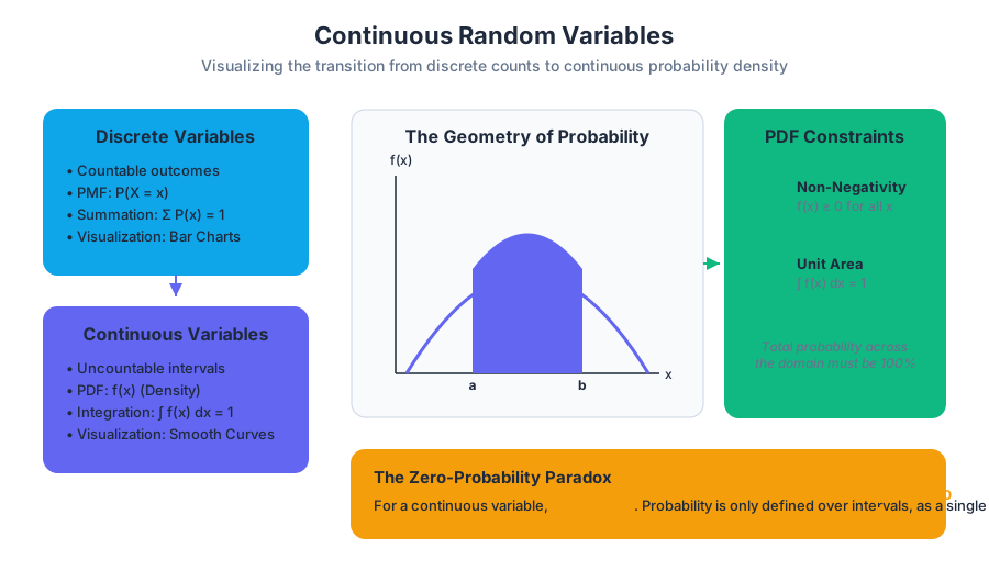
The behavior of a continuous random variable is described by a Probability Density Function (PDF), denoted as $f(x)$. Unlike discrete probability mass functions, the value of $f(x)$ at any specific point does not represent a probability. Instead, it represents the "density" of probability at that point.
The Fundamental Constraints
For a function to qualify as a valid PDF for a continuous random variable $X$, it must satisfy two rigorous mathematical conditions:
- Non-negativity: $f(x) \ge 0$ for all possible values of $x$. Probability density cannot be negative.
- Unit Area: The total area under the curve across the entire domain of $X$ must equal exactly 1. Mathematically: $\int_{-\infty}^{\infty} f(x) dx = 1$.
Area Under the Curve (AUC)
In the continuous domain, the probability that $X$ falls between two values $a$ and $b$ is defined as the area under the PDF curve between those two points.
The Zero-Probability Paradox: For any continuous random variable, the probability that $X$ is exactly equal to a specific value $c$ is zero ($P(X = c) = 0$). This is because the area of a line segment with width zero is zero. Consequently, $P(a \le X \le b)$ is identical to $P(a < X < b)$.
| Feature | Discrete Random Variables | Continuous Random Variables |
|---|---|---|
| Values | Countable (integers, finite sets) | Uncountable (intervals, real numbers) |
| Function Type | Probability Mass Function (PMF) | Probability Density Function (PDF) |
| Probability at a point | $P(X=x) = f(x)$ | $P(X=x) = 0$ |
| Total Sum/Integral | $\sum P(x) = 1$ | $\int f(x) dx = 1$ |
| Visualization | Histograms / Bar Charts | Smooth Curves (Density Plots) |
The Uniform Distribution
The Uniform Distribution is the simplest continuous distribution, often referred to as the "rectangular distribution." It models a scenario where every interval of the same length within the distribution's domain is equally likely.
Mathematical Definition
A continuous random variable $X$ follows a uniform distribution between $a$ and $b$, denoted as $X \sim U(a, b)$, if its PDF is:
$$f(x) = \begin{cases} \frac{1}{b - a} & \text{for } a \le x \le b \ 0 & \text{otherwise} \end{cases}$$
Key Parameters and Statistics
The uniform distribution is defined by its boundaries $a$ (minimum) and $b$ (maximum).
| Statistic | Formula | Description |
|---|---|---|
| Mean ($\mu$) | $\frac{a + b}{2}$ | The midpoint of the interval. |
| Variance ($\sigma^2$) | $\frac{(b - a)^2}{12}$ | Measures the spread relative to the interval width. |
| Standard Deviation ($\sigma$) | $\sqrt{\frac{(b - a)^2}{12}}$ | The square root of the variance. |
| CDF $F(x)$ | $\frac{x - a}{b - a}$ | The cumulative probability from $a$ to $x$. |
The Exponential Distribution
While the Uniform distribution deals with "where," the Exponential Distribution is primarily concerned with "when." It is frequently used to model the time elapsed between independent events occurring at a constant average rate. Common applications include the time between radioactive decays, the time until a lightbulb fails, or the time between customer arrivals in a queue.
The Rate Parameter ($\lambda$)
The distribution is characterized by the rate parameter $\lambda$ (lambda), which represents the average number of events per unit of time. If a system receives 10 requests per second, $\lambda = 10$.
Probability Density Function
The PDF of an exponential distribution is defined for $x \ge 0$:
$$f(x) = \lambda e^{-\lambda x}$$
The Memoryless Property
Perhaps the most counter-intuitive and significant feature of the exponential distribution is that it is memoryless.
Definition: A random variable $X$ is memoryless if $P(X > s + t \mid X > s) = P(X > t)$ for all $s, t \ge 0$.
In practical terms, if the lifespan of a component is exponentially distributed, the probability that it will last another 100 hours is the same whether it is brand new or has already been running for 500 hours. The component does not "age" in a way that affects its immediate probability of failure.
Derivation of the Cumulative Distribution Function (CDF)
To find the probability that an event occurs within a certain time $x$, we integrate the PDF.
% Mathematical Derivation of the Exponential CDF
F(x) = P(X \le x) = \int_{0}^{x} \lambda e^{-\lambda t} dt
% Applying the fundamental theorem of calculus:
F(x) = [ -e^{-\lambda t} ]_{0}^{x}
F(x) = (-e^{-\lambda x}) - (-e^{0})
F(x) = 1 - e^{-\lambda x}
Comparison: Exponential vs. Poisson
It is vital to distinguish between the Poisson and Exponential distributions, as they are two sides of the same coin.
| Distribution | Type | What it Measures | Parameter |
|---|---|---|---|
| Poisson | Discrete | The number of events in a fixed interval. | $\mu$ or $\lambda$ (Mean count) |
| Exponential | Continuous | The time between those events. | $\lambda$ (Rate) or $m = 1/\lambda$ (Mean time) |
Practical Application: Reliability Engineering
In systems engineering, we often use the exponential distribution to model the Mean Time Between Failures (MTBF). If a hard drive has an MTBF of 500,000 hours, the rate $\lambda$ is $1/500,000$.
Cumulative Distribution Functions (CDF) and Percentiles
The Cumulative Distribution Function (CDF), $F(x)$, is the probability that the random variable $X$ is less than or equal to $x$. For continuous variables, the CDF is the running integral of the PDF.
Calculating Percentiles
The $k$-th percentile is the value $x$ such that $P(X < x) = k/100$.
- For the Uniform Distribution, the median (50th percentile) is simply the mean $\frac{a+b}{2}$.
- For the Exponential Distribution, the median is $\frac{\ln(2)}{\lambda}$, which is approximately $0.693 \times \text{mean}$. Note that for exponential distributions, the median is always smaller than the mean due to the long right tail.
Summary of CDFs
| Distribution | CDF Formula $F(x)$ | Solving for $x$ (Percentile) |
|---|---|---|
| Uniform | $\frac{x-a}{b-a}$ | $x = a + p(b-a)$ |
| Exponential | $1 - e^{-\lambda x}$ | $x = \frac{-\ln(1-p)}{\lambda}$ |
Common Pitfalls and Misconceptions
1. Confusing $f(x)$ with $P(X=x)$
In a continuous distribution, $f(x)$ can be greater than 1. For example, in $U(0, 0.5)$, the density $f(x) = 1/(0.5 - 0) = 2$. This is not a probability; the probability is the area, which will never exceed 1.
2. The Memoryless Property Misapplication
The memoryless property only applies to the Exponential distribution. It does not apply to the Normal distribution, nor does it apply to human aging or mechanical wear-and-tear that involves physical degradation (which usually follows a Weibull distribution).
3. Endpoint Inclusion
Beginners often worry whether to use $P(X < x)$ or $P(X \le x)$. In continuous probability, the boundary point has zero width and zero probability, so the choice of inequality ($<$ vs $\le$) is mathematically irrelevant.
4. The "Average" Trap
In skewed distributions like the Exponential, the "average" (mean) is not the "typical" (median) value. If the mean time to failure is 100 days, more than 50% of units will likely fail before 100 days because the mean is pulled higher by a few long-lasting outliers.
Advanced Extensions: The Relationship to the Normal Distribution
While Uniform and Exponential distributions are foundational, they often serve as building blocks for the Normal (Gaussian) Distribution. According to the Central Limit Theorem, the sum of many independent continuous random variables (regardless of their original distribution) tends toward a Normal distribution.
Furthermore, the Exponential distribution is a special case of the Gamma Distribution (where we wait for $n$ events instead of just one) and the Weibull Distribution (which allows the failure rate to increase or decrease over time).
Summary of Key Relationships
- Uniform is the distribution of "maximum uncertainty" within a range.
- Exponential is the distribution of "waiting time" for a random event.
- PDF is the shape; CDF is the accumulated area.
- Integration replaces summation when moving from discrete to continuous.
- Continuous Random Variable: A variable with an infinite number of possible values in an interval.
- PDF (Probability Density Function): A function $f(x)$ used to calculate probabilities via the area under its curve.
- CDF (Cumulative Distribution Function): $F(x) = P(X \le x)$, representing the area under the PDF to the left of $x$.
- Uniform Distribution: A distribution where all equal-length intervals are equally likely.
- Exponential Distribution: A distribution modeling the time between independent events at a constant rate.
- Memoryless Property: The probability of a future event occurring is independent of how much time has already passed.
- Lambda ($\lambda$): The rate parameter in an exponential distribution (events per unit time).
- Area Under the Curve: The geometric representation of probability for continuous variables.
- Why is $P(X = 5)$ equal to 0 for a continuous random variable?
- If $X \sim U(10, 50)$, what is the height of the density function $f(x)$?
- A call center receives 4 calls per hour. What is the mean time between calls, and which distribution models this?
- True or False: If a component's life is exponentially distributed and it has lasted 50 hours, it is more likely to fail in the next hour than a brand-new component.
- How do you calculate the 90th percentile of a $U(0, 100)$ distribution?
- What is the total area under any valid PDF?
DeepWiki Study Guide: Continuous Random Variables
Primary Objective: Transition from discrete counting to continuous measurement using calculus-based probability concepts.
Key Formulas to Memorize:
- Uniform PDF: $1/(b-a)$
- Uniform Mean: $(a+b)/2$
- Exponential PDF: $\lambda e^{-\lambda x}$
- Exponential Mean: $1/\lambda$
- Exponential CDF: $1 - e^{-\lambda x}$
Conceptual Check:
- Can you explain why the PDF value $f(x)$ is not a probability?
- Can you derive the median of an exponential distribution using the CDF?
- Do you understand the relationship between the Poisson rate and Exponential time?
Practical Skills:
- Be able to calculate the probability of an interval $P(a < X < b)$ for both Uniform and Exponential distributions.
- Be able to identify real-world scenarios (e.g., bus arrivals, radioactive decay) and map them to the correct distribution.
- Recognize the "Memoryless" property in word problems to simplify conditional probability calculations.
Further Reading:
- OpenStax Introductory Statistics 2e: Chapter 5 (Continuous Random Variables).
- Inverse Transform Sampling: Explore how computers generate non-uniform random numbers.
- The Weibull Distribution: Learn how to model systems that do have "memory" or wear-out effects.
Source Materials
Study Introductory Statistics on Lykke
This course page is free to open: signed out, you can read its first two sections, and signing in, on any plan, opens the rest. The free Lykke Chrome extension syncs your own Canvas courses, so ChatGPT, Claude and Muse can answer from your classes and deadlines. It only reads Canvas.
Add the free extensionSign in to open every sectionAll sections of Introductory Statistics · Browse more course pages