From the free course Introductory Statistics on Lykke
Confidence Intervals
Key concepts: Margin of Error · Confidence Level · Point Estimate · T-Distribution
Estimating population parameters using intervals rather than single points.
Confidence Intervals
In frequentist statistics, we are often tasked with estimating an unknown population parameter (such as a mean $\mu$ or a proportion $p$) based on a finite sample. While a Point Estimate provides a single "best guess," it offers no information regarding the precision or reliability of that guess. A Confidence Interval (CI) addresses this by providing a range of plausible values for the parameter, accompanied by a quantitative measure of certainty.
The Philosophy of Interval Estimation
The transition from point estimation to interval estimation represents a shift from "finding a value" to "quantifying uncertainty." If we report that the average height of a population is 175 cm, we provide no context on whether that estimate is based on five people or five thousand. A confidence interval contextualizes the estimate by incorporating the variability of the data and the size of the sample.
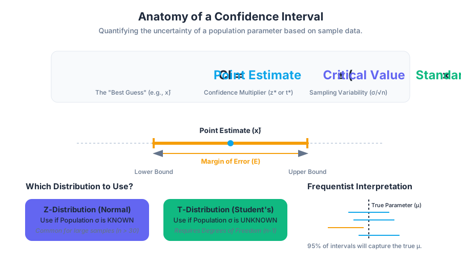
Definition: A Confidence Interval is an interval of the form $(\text{point estimate} - \text{margin of error}, \text{point estimate} + \text{margin of error})$. It is designed to contain the true population parameter with a specified probability, known as the Confidence Level.
The Frequentist Interpretation
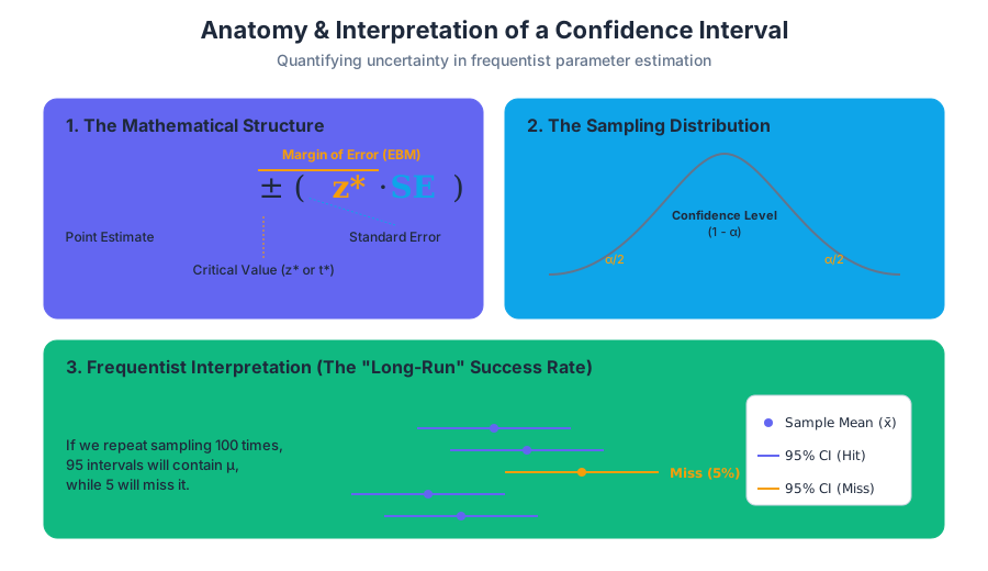
A common misconception is that a 95% confidence interval has a 95% probability of containing the true parameter. Technically, in frequentist statistics, the population parameter is a fixed (though unknown) constant. It is the interval that is the random variable.
- Correct Interpretation: If we were to repeat the sampling process 100 times and calculate a 95% confidence interval for each sample, approximately 95 of those intervals would contain the true population parameter.
Key Components of a Confidence Interval
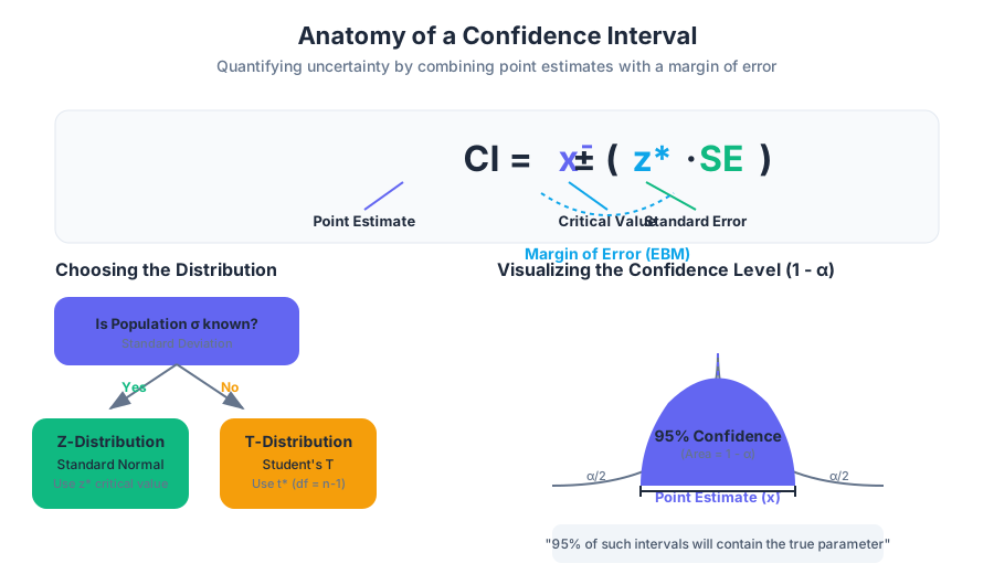
To construct an interval, four primary components must be synthesized: the point estimate, the confidence level, the standard error, and the critical value.
| Component | Symbol | Description |
|---|---|---|
| Point Estimate | $\bar{x}$ or $\hat{p}$ | The sample statistic used as the center of the interval. |
| Confidence Level | $1 - \alpha$ | The success rate of the method (usually 0.90, 0.95, or 0.99). |
| Alpha (Significance) | $\alpha$ | The probability that the interval does not contain the parameter. |
| Standard Error | $SE$ | The standard deviation of the sampling distribution of the statistic. |
| Critical Value | $z^$ or $t^$ | The number of standard errors move away from the mean to capture the desired area. |
| Margin of Error | $EBM$ or $E$ | The product of the critical value and the standard error ($z^* \times SE$). |
1. The Point Estimate
The Point Estimate is the specific value calculated from the sample. For a population mean $\mu$, the point estimate is the sample mean $\bar{x}$. For a population proportion $P$, it is the sample proportion $\hat{p} = x/n$.
2. The Confidence Level ($1 - \alpha$)
The Confidence Level represents the long-term success rate of the estimation procedure. If $1 - \alpha = 0.95$, then $\alpha = 0.05$. This $\alpha$ is the "area in the tails" of the probability distribution that we are willing to exclude.
3. The Margin of Error (EBM)
Also known as the Error Bound for a Population Mean (EBM), this is the distance from the point estimate to the interval boundaries. It is the "plus-minus" part of the statistic.
The Mathematics of the Interval
The construction of a confidence interval relies on the Central Limit Theorem (CLT), which states that for a sufficiently large sample size, the sampling distribution of the mean will be approximately normal, regardless of the population's distribution.
Case A: Known Population Standard Deviation ($\sigma$)
When the population standard deviation $\sigma$ is known, we use the Z-distribution (Standard Normal).
CI = \bar{x} \pm z_{\alpha/2} \left( \frac{\sigma}{\sqrt{n}} \right)
Case B: Unknown Population Standard Deviation ($s$)
In practice, $\sigma$ is rarely known. We must estimate it using the sample standard deviation $s$. This introduces extra uncertainty, especially in small samples. To account for this, we use the Student's T-Distribution.
CI = \bar{x} \pm t_{\alpha/2, df} \left( \frac{s}{\sqrt{n}} \right)
Where $df = n - 1$ (degrees of freedom).
The Student's T-Distribution
Developed by William Sealy Gosset (under the pseudonym "Student") while working for the Guinness Brewery, the T-distribution is essential when sample sizes are small ($n < 30$) or the population variance is unknown.
Characteristics of the T-Distribution
- Bell-shaped and Symmetric: Like the Z-distribution, it is centered at zero.
- Heavier Tails: The T-distribution has more probability in its tails than the Z-distribution. This reflects the added uncertainty of estimating $\sigma$ with $s$.
- Degrees of Freedom ($df$): As $n$ increases, the T-distribution approaches the Standard Normal distribution. With infinite degrees of freedom, $t = z$.
| Sample Size ($n$) | $df$ | Critical Value ($t^*$) for 95% CI | Critical Value ($z^*$) for 95% CI |
|---|---|---|---|
| 5 | 4 | 2.776 | 1.960 |
| 10 | 9 | 2.262 | 1.960 |
| 30 | 29 | 2.045 | 1.960 |
| 100 | 99 | 1.984 | 1.960 |
| $\infty$ | $\infty$ | 1.960 | 1.960 |
Calculating a Confidence Interval
To calculate a confidence interval for a mean where the population standard deviation is unknown, we follow a systematic algorithmic approach.
Confidence Intervals for Proportions
When dealing with categorical data (e.g., "Yes/No" surveys), we estimate the population proportion $P$. The point estimate is $\hat{p} = x/n$.
Requirements for Normality
To use the Normal approximation for proportions, the Success-Failure Condition must be met:
- $np \geq 10$
- $n(1-p) \geq 10$
Derivation of the Proportion Interval
The standard error for a proportion is $\sqrt{\frac{\hat{p}(1-\hat{p})}{n}}$.
\text{Step 1: Identify } \hat{p} = \frac{x}{n}
\text{Step 2: Identify } \hat{q} = 1 - \hat{p}
\text{Step 3: Calculate } SE = \sqrt{\frac{\hat{p}\hat{q}}{n}}
\text{Step 4: Find } z_{\alpha/2} \text{ for the confidence level.}
\text{Step 5: } CI = \hat{p} \pm z_{\alpha/2} \cdot SE
Factors Affecting Interval Width
The width of a confidence interval is a proxy for the precision of our estimate. A narrower interval indicates higher precision.
| Factor | Change | Effect on Interval Width | Reason |
|---|---|---|---|
| Confidence Level | Increase (90% $\to$ 99%) | Wider | To be more certain, we must include more possible values. |
| Sample Size ($n$) | Increase | Narrower | Larger samples reduce the standard error ($\sqrt{n}$ is in the denominator). |
| Variability ($s$ or $\sigma$) | Increase | Wider | More "noise" in the data makes the estimate less certain. |
Determining Required Sample Size
One of the most practical applications of CI theory is determining how many subjects are needed for a study before data collection begins. This is done by specifying a desired Margin of Error ($E$).
For Means:
To solve for $n$, we rearrange the EBM formula: $E = z \frac{\sigma}{\sqrt{n}} \implies \sqrt{n} = \frac{z \sigma}{E} \implies n = \left( \frac{z \sigma}{E} \right)^2$
For Proportions:
$n = \frac{z^2 \hat{p} \hat{q}}{E^2}$ Note: If no preliminary $\hat{p}$ is known, use $0.5$ as a conservative estimate, as it maximizes the required $n$.
Common Pitfalls and Misconceptions
1. The "Probability" Trap
As noted earlier, once an interval is calculated (e.g., [10, 20]), the probability that the parameter is in that specific interval is either 0 or 1. The "95%" refers to the reliability of the process, not the specific result.
2. Over-reliance on $n=30$
While 30 is a common rule of thumb for the Central Limit Theorem, it is not a magic number. If the underlying population is extremely skewed or contains heavy outliers, much larger samples may be required for the Z or T distributions to be valid.
3. Standard Deviation vs. Standard Error
- Standard Deviation ($s$): Measures the dispersion of individual data points.
- Standard Error ($SE$): Measures the dispersion of the sample mean from the population mean. Confidence intervals always use the Standard Error.
4. Confusing CI with Prediction Intervals
A Confidence Interval estimates where the mean of the population lies. A Prediction Interval estimates where a single future observation will lie. Prediction intervals are significantly wider because they must account for both the uncertainty in the mean and the inherent variability of individuals.
Advanced Variations
Bootstrap Confidence Intervals
When the underlying distribution is unknown and the sample size is small, we can use Bootstrapping. This involves resampling the data with replacement thousands of times to generate an empirical sampling distribution. The 2.5th and 97.5th percentiles of this distribution form the 95% CI.
Bayesian Credible Intervals
Unlike Frequentist CIs, Bayesian Credible Intervals do allow for probability statements about the parameter. By combining a "Prior" belief with the "Likelihood" of the data, Bayesians produce a "Posterior" distribution. A 95% Credible Interval is the range that contains 95% of the posterior probability.
Source Materials
Study Introductory Statistics on Lykke
This course page is free to open: signed out, you can read its first two sections, and signing in, on any plan, opens the rest. The free Lykke Chrome extension syncs your own Canvas courses, so ChatGPT, Claude and Muse can answer from your classes and deadlines. It only reads Canvas.
Add the free extensionSign in to open every sectionAll sections of Introductory Statistics · Browse more course pages