From the free course Introductory Biology on Lykke
Genetic Mapping and Linkage
Key concepts: Recombination Frequency · Centimorgans (cM) · Three-point Cross · SNP Mapping · Yeast Tetrad Analysis
Advanced genetics focusing on gene linkage, recombination frequencies, and mapping techniques.
Genetic Mapping and Linkage
The fundamental law of Mendelian genetics is the Law of Independent Assortment, which posits that alleles of different genes segregate independently during gamete formation. However, as the field of genetics matured in the early 20th century, researchers like Thomas Hunt Morgan and Alfred Sturtevant discovered that certain genes are "linked"—they travel together on the same chromosome.
Genetic Mapping is the process of determining the relative positions of genes on a chromosome based on how often they are separated by recombination. This section explores the transition from qualitative inheritance to quantitative spatial mapping, providing the mathematical and experimental framework for understanding the architecture of the genome.
The Physical Basis of Linkage
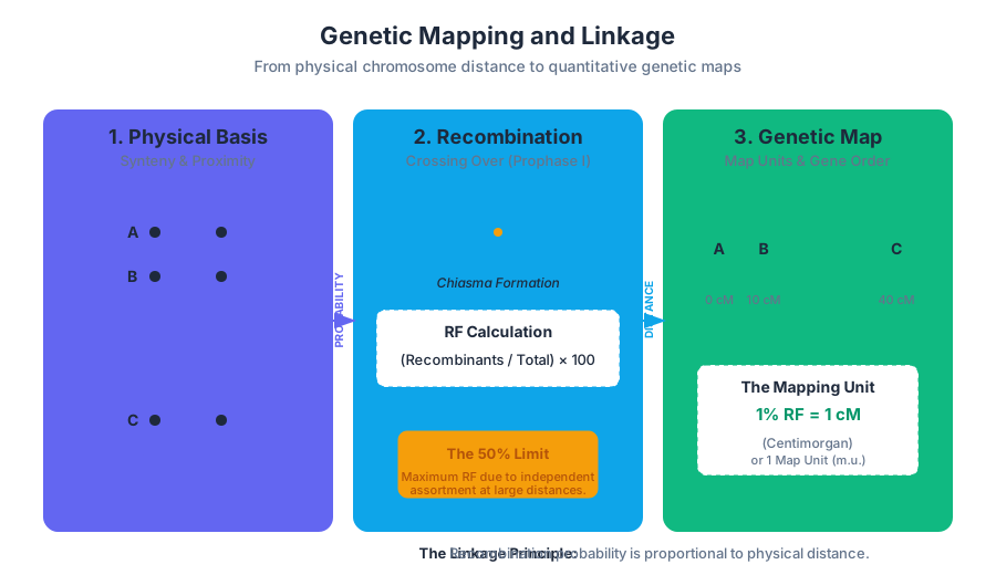
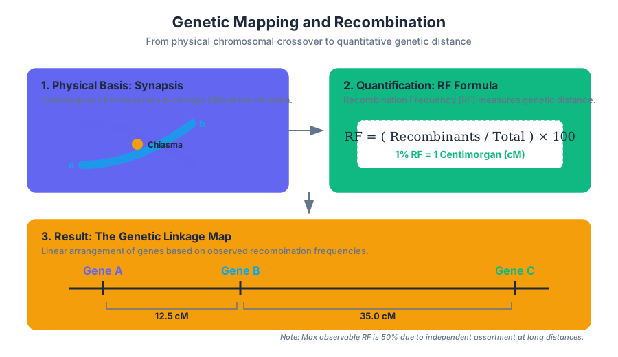
Linkage occurs when two loci are located on the same physical DNA molecule (chromosome). During Prophase I of meiosis, homologous chromosomes undergo synapsis, forming a synaptonemal complex where genetic material is exchanged. This process, known as crossing over or recombination, is the only mechanism by which alleles on the same chromosome can be uncoupled.
The Linkage Principle: The probability of a crossover occurring between two loci is proportional to the physical distance between them. The further apart two genes are, the more likely a recombination event will occur in the intervening space.
Recombination Frequency (RF)
The Recombination Frequency is the primary metric used to estimate genetic distance. It is calculated as the ratio of recombinant offspring to the total number of offspring.
$$RF = \frac{\text{Number of Recombinant Progeny}}{\text{Total Number of Progeny}} \times 100$$
By convention, an $RF$ of 1% is defined as one Centimorgan (cM), also known as a map unit (m.u.).
Recombination and Map Distance
While $RF$ is a reliable proxy for distance at short intervals, it is not perfectly linear over long distances. This is because multiple crossovers can occur between two distant genes. A double crossover between two genes restores the original parental allele combination, making the offspring appear as "non-recombinants" even though recombination occurred.
The 50% Limit
Even if two genes are at opposite ends of a very long chromosome, the maximum observed $RF$ is 50%. This is because recombination involves only two of the four chromatids in a meiotic bivalent. At great distances, the genes assort as if they were on different chromosomes (independent assortment).
| Parameter | Definition | Typical Range |
|---|---|---|
| Linkage | Genes on the same chromosome | 0 - 50 cM |
| Synteny | Genes physically on the same chromosome | Any distance |
| Map Unit (cM) | 1% Recombination Frequency | 0.1 - 50 cM |
| Physical Distance | Base pairs (bp) | Varies by species (e.g., ~1Mb/cM in humans) |
Calculating Recombination in a Two-Point Cross
To calculate the distance between two genes, $A$ and $B$, we perform a testcross. We cross a double heterozygote ($AaBb$) with a double homozygous recessive ($aabb$).
The Three-Point Cross
The Three-Point Cross is the definitive method for determining the order and distance of three linked genes ($A, B, C$) in a single experiment. It is superior to two-point crosses because it allows for the detection of double crossovers (DCOs), which are the rarest classes of offspring.
Step-by-Step Logic
- Identify Parental Classes: The two most frequent phenotypic classes are the parentals (no crossovers).
- Identify Double Crossover (DCO) Classes: The two least frequent classes result from two recombination events.
- Determine Gene Order: Compare the parentals to the DCOs. The gene that "swaps" relative to the other two in the DCO classes is the gene in the middle.
- Calculate SCO Distances: Sum the Single Crossovers (SCO) and DCOs for each interval and divide by the total.
Interference and Coincidence
In most organisms, a crossover in one region of the chromosome reduces the probability of a second crossover nearby. This phenomenon is called chromosomal interference.
Coefficient of Coincidence ($C$): The ratio of observed DCOs to expected DCOs. $$C = \frac{\text{Observed DCO Frequency}}{\text{Expected DCO Frequency}}$$ Interference ($I$): $I = 1 - C$. If $I = 1$, interference is complete (no DCOs). If $I = 0$, crossovers are independent.
% Mathematical derivation of Expected DCOs
\text{Expected DCO} = RF(\text{Interval 1}) \times RF(\text{Interval 2}) \times \text{Total Progeny}

% Example:
% Interval A-B = 0.10 (10 cM)
% Interval B-C = 0.20 (20 cM)
% Total Progeny = 1000
\text{Expected DCO} = 0.10 \times 0.20 \times 1000 = 20
| Offspring Phenotype | Count | Class |
|---|---|---|
| $v\ cv\ ct$ | 580 | Parental |
| $+\ +\ +$ | 592 | Parental |
| $v\ +\ +$ | 45 | SCO (v-cv) |
| $+\ cv\ ct$ | 40 | SCO (v-cv) |
| $v\ cv\ +$ | 89 | SCO (cv-ct) |
| $+\ +\ ct$ | 94 | SCO (cv-ct) |
| $v\ +\ ct$ | 3 | DCO |
| $+\ cv\ +$ | 5 | DCO |
Yeast Tetrad Analysis
In fungi like Saccharomyces cerevisiae, the four products of a single meiosis are held together in a sac called an ascus. Analyzing these tetrads allows geneticists to look directly at the results of recombination without the statistical noise of random fertilization.
Tetrad Types
When crossing two strains ($AB \times ab$), three types of tetrads can be produced:
- Parental Ditype (PD): Contains four parental spores ($2 AB, 2 ab$).
- Non-Parental Ditype (NPD): Contains four recombinant spores ($2 Ab, 2 aB$). This occurs via a four-strand double crossover.
- Tetratype (TT): Contains two parental and two recombinant spores ($1 AB, 1 ab, 1 Ab, 1 aB$). This occurs via a single crossover.
Mapping Formula for Tetrads
Linkage is identified when $PD \gg NPD$. The distance is calculated using the formula:
$$cM = \frac{1/2 TT + 3 NPD}{\text{Total Tetrads}} \times 100$$
The $3 \times NPD$ term is a correction factor that accounts for multiple crossovers that result in NPDs.
| Relationship | Ratio | Conclusion |
|---|---|---|
| Independent Assortment | $PD \approx NPD$ | Genes on different chromosomes |
| Linkage | $PD \gg NPD$ | Genes on the same chromosome |
| Centromere Linkage | Low $TT$ frequency | Genes close to their respective centromeres |
SNP Mapping and Modern Genomics
In modern human genetics, we rarely use phenotypic markers like "curly hair" or "eye color" for mapping. Instead, we use Single Nucleotide Polymorphisms (SNPs)—single-base variations in the DNA sequence.
LOD Scores
Because human families are small, we cannot use simple recombination frequencies to map disease genes. Instead, we use the LOD Score (Logarithm of the Odds).
LOD Score Definition: The log-ratio of the likelihood that two loci are linked at a specific distance ($\theta$) versus the likelihood that they are unlinked ($\theta = 0.5$). $$LOD = \log_{10} \left( \frac{\text{Likelihood of linkage at } \theta}{\text{Likelihood of independent assortment}} \right)$$
- LOD > 3.0: Statistically significant evidence for linkage (1000:1 odds).
- LOD < -2.0: Evidence against linkage.
Genome-Wide Association Studies (GWAS)
GWAS leverages Linkage Disequilibrium (LD)—the non-random association of alleles at different loci. If a specific SNP is consistently found in patients with a disease, that SNP is likely "linked" to the causal mutation.
Mapping Functions: Haldane vs. Kosambi
As mentioned, $RF$ is not additive over long distances. Mapping functions translate observed $RF$ into more accurate map distances (cM) by modeling the probability of multiple crossovers.
- Haldane Mapping Function: Assumes no interference. Crossovers occur randomly according to a Poisson distribution. $$d = -\frac{1}{2} \ln(1 - 2 \cdot RF)$$
- Kosambi Mapping Function: Accounts for interference, assuming that one crossover inhibits another nearby. This is generally more accurate for most eukaryotic chromosomes. $$d = \frac{1}{4} \ln \left( \frac{1 + 2 \cdot RF}{1 - 2 \cdot RF} \right)$$
Common Pitfalls in Mapping
- Underestimating Distance: Failing to account for double crossovers leads to "shorter" maps. This is why three-point crosses are preferred over two-point crosses.
- Sex-Specific Differences: In many species, recombination rates differ between sexes. In Drosophila, recombination occurs only in females. In humans, females generally have higher recombination rates than males.
- Hotspots and Coldspots: Recombination is not uniform across the chromosome. Centromeres are typically recombination "coldspots," while other regions are "hotspots." Consequently, genetic distance (cM) does not always map linearly to physical distance (bp).
Source Materials
Study Introductory Biology on Lykke
This course page is free to open: signed out, you can read its first two sections, and signing in, on any plan, opens the rest. The free Lykke Chrome extension syncs your own Canvas courses, so ChatGPT, Claude and Muse can answer from your classes and deadlines. It only reads Canvas.
Add the free extensionSign in to open every sectionAll sections of Introductory Biology · Browse more course pages