From the free course Intro to Python Fundamentals on Lykke
Unit 3: Loops and Simulations
Key concepts: While loops · For loops with range · Module imports (random) · Loop control (break and continue) · Population dynamics simulations
Focuses on automating repetitive tasks and simulating complex phenomena using loops.
Unit 3: Loops and Simulations
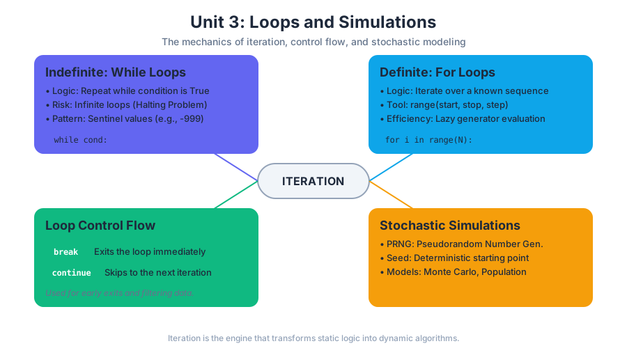
Iteration is the engine of computation. While the previous units focused on state (variables) and selection (conditionals), Unit 3 introduces the ability to repeat logic dynamically. In computer science, we transition from writing linear scripts to designing algorithms—procedures that can handle arbitrary scales of data and time.
This unit explores the two primary forms of iteration: indefinite iteration (where the number of repetitions is unknown at the start) and definite iteration (where we iterate over a known sequence). We will then synthesize these concepts with stochasticity (randomness) to build simulations of complex systems, such as population dynamics and Monte Carlo models.
3.1 Indefinite Iteration: The While Loop
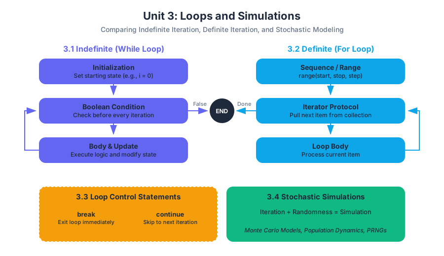
The while loop is the most fundamental looping construct. It functions as a "repeated if statement." As long as a specified Boolean condition evaluates to True, the code block within the loop executes. Once the condition becomes False, the program pointer moves to the next instruction outside the loop.
3.1.1 Mechanics and Syntax
A while loop consists of a loop header and a loop body. The header contains the condition, and the body contains the instructions.
The Halting Problem: In theoretical computer science, determining whether a given program will eventually stop (halt) or run forever is undecidable. When writing
whileloops, the burden is on the programmer to ensure the loop condition eventually evaluates toFalse.
| Component | Role | Risk if Mismanaged |
|---|---|---|
| Initialization | Setting the starting state of the control variable. | Uninitialized variable error. |
| Condition | The Boolean expression checked before every iteration. | Logic error leading to zero iterations. |
| Update | Modifying the state so the condition eventually fails. | Infinite Loop: The program hangs indefinitely. |
3.1.2 Implementation: The Sentinel Pattern
A common use for while loops is processing user input or data streams where the end-point is marked by a specific value, known as a sentinel.
# Implementation of a robust data accumulator with a sentinel value
def collect_sensor_data():
    data_points = []
    sentinel = -999.0  # Value indicating end of stream

    print(f"Enter sensor readings (type {sentinel} to stop):")

    while True:
        try:
            raw_input = input("> ")
            val = float(raw_input)

            if val == sentinel:
                break  # Exit loop immediately

            data_points.append(val)

        except ValueError:
            print("Invalid input. Please enter a numeric value.")

    return data_points

# Calculate average from the collected data
readings = collect_sensor_data()
if readings:
    print(f"Mean Reading: {sum(readings) / len(readings):.2f}")
3.2 Definite Iteration: For Loops and the Range Object
While while loops are powerful for state-based repetition, for loops are the standard for iterating over a sequence of values. In Python, the for loop is an iterator-based construct, meaning it pulls items from a collection one by one.
3.2.1 The range() Function
The range() function is a built-in generator that produces a sequence of integers. It is highly memory-efficient because it does not store the entire list of numbers in memory; instead, it calculates the next number on demand.
The range(start, stop, step) function follows these mathematical rules:
- Start: Inclusive.
- Stop: Exclusive (the loop stops before reaching this value).
- Step: The increment between values (can be negative for counting down).
Algorithm: Range Sequence Generation
Input: start (a), stop (b), step (s)
Output: A sequence S where S_i = a + i*s
Constraint:
    If s > 0: a + i*s < b
    If s < s: a + i*s > b
3.2.2 Comparison of Range Parameters
| Syntax | Sequence Produced | Use Case |
|---|---|---|
range(5) |
0, 1, 2, 3, 4 | Simple repetition $N$ times. |
range(1, 6) |
1, 2, 3, 4, 5 | Iterating through 1-based indices. |
range(0, 10, 2) |
0, 2, 4, 6, 8 | Iterating through even numbers. |
range(10, 0, -1) |
10, 9, 8, ..., 1 | Counting down (e.g., a timer). |
3.3 Loop Control: Break and Continue
Sometimes, the standard entry/exit logic of a loop is insufficient. We use control flow statements to alter the loop's execution path mid-stream.
break: Immediately terminates the innermost loop. Execution resumes at the first statement after the loop block.continue: Skips the remainder of the current loop body and jumps back to the header for the next iteration (re-evaluating the condition).
3.2.3 Low-Level Logic Comparison
To understand how these work at the hardware level, we can look at how a high-level for loop with a break might be represented in a lower-level language like C, which maps more closely to assembly jumps.
#include <stdio.h>

// Demonstrating loop control at a low level
int main() {
    int target = 7;

    // For loop: (initialization; condition; increment)
    for (int i = 0; i < 10; i++) {
        if (i % 2 == 0) {
            // 'continue' equivalent: jump to increment
            continue;
        }

        if (i == target) {
            // 'break' equivalent: jump out of loop
            break;
        }

        printf("Processing odd number: %d\n", i);
    }

    return 0;
}
3.4 Stochasticity and the random Module
Simulations require unpredictability. Since computers are deterministic machines, they use Pseudorandom Number Generators (PRNGs). These are mathematical algorithms that produce a sequence of numbers that appear random but are actually determined by an initial value called a seed.
3.4.1 Key Functions in random
| Function | Output Type | Description |
|---|---|---|
random.random() |
Float | Returns a value in the range $[0.0, 1.0)$. |
random.randint(a, b) |
Integer | Returns a value in the range $[a, b]$ (inclusive). |
random.uniform(a, b) |
Float | Returns a value in the range $[a, b]$. |
random.choice(seq) |
Element | Returns a random element from a non-empty sequence. |
Pro-Tip: For scientific simulations, always set a seed using
random.seed(value). This ensures your results are reproducible, allowing other researchers to generate the exact same "random" sequence.
3.5 Population Dynamics and Simulations
A simulation is a computational model of a real-world process. In biology and sociology, we often simulate population dynamics to predict how a group of organisms changes over time based on birth rates, death rates, and environmental carrying capacity.
3.5.1 The Discrete-Time Model
In a loop-based simulation, we treat time as a series of discrete "steps" (e.g., years or generations). At each step, we apply a set of rules to update the state.
The Malthusian Growth Formula: $$P_{t+1} = P_t + (r \times P_t)$$ Where:
- $P_t$ is the population at time $t$.
- $r$ is the growth rate (birth rate - death rate).
3.5.2 Complex Simulation: Logistic Growth with Stochasticity
In reality, populations don't grow forever. They are limited by a Carrying Capacity (K). Furthermore, random events (famine, disease) introduce variance.
import random

def simulate_population(initial_pop, growth_rate, carrying_capacity, years):
    """
    Simulates population growth using the Logistic Model with
    stochastic environmental shocks.
    """
    population = initial_pop
    history = [initial_pop]

    print(f"{'Year':<5} | {'Population':<12} | {'Event'}")
    print("-" * 35)

    for year in range(1, years + 1):
        # 1. Calculate deterministic growth (Logistic Equation)
        # Growth slows as population approaches K
        growth = growth_rate * population * (1 - population / carrying_capacity)

        # 2. Introduce Stochasticity (Random Environmental Shock)
        # 10% chance of a "bad year" where 20% of the population is lost
        event = "Stable"
        if random.random() < 0.10:
            growth -= (population * 0.20)
            event = "Famine!"

        population += int(growth)

        # Ensure population doesn't drop below zero
        population = max(0, population)
        history.append(population)

        print(f"{year:<5} | {population:<12} | {event}")

        if population == 0:
            print("Extinction event occurred.")
            break

    return history

# Execution
results = simulate_population(initial_pop=50, growth_rate=0.5, carrying_capacity=1000, years=50)
3.6 Complexity and Nested Loops
When a loop is placed inside another loop, it is called a nested loop. These are essential for working with multi-dimensional data (like grids or matrices) but can lead to performance bottlenecks.
3.6.1 Big O Notation and Performance
The efficiency of a loop is often measured in Big O notation, which describes how the execution time grows as the input size ($n$) increases.
| Structure | Complexity | Description |
|---|---|---|
| Single Loop | $O(n)$ | Linear time. If $n$ doubles, time doubles. |
| Nested Loop (2 levels) | $O(n^2)$ | Quadratic time. If $n$ doubles, time quadruples. |
| Nested Loop (3 levels) | $O(n^3)$ | Cubic time. Common in 3D simulations. |
3.6.2 Example: Coordinate Grid Generation
To simulate a 2D environment (like a forest or a game map), we use nested loops to iterate over $x$ and $y$ coordinates.
# Example of how a shell script might invoke a Python simulation
# with different parameters to conduct a sensitivity analysis.

for rate in 0.1 0.2 0.3 0.4 0.5; do
    echo "Running simulation with growth rate: $rate"
    python3 population_sim.py --rate $rate --output "results_$rate.csv"
done

echo "All simulations complete. Analyzing data..."
3.7 Common Pitfalls in Loop Design
- Off-by-One Errors: Using
range(10)when you need the number 10 included. Remember thatstopis exclusive. - Modifying the Iterator: Never add or remove items from a list while you are iterating over it with a
forloop. This leads to skipped elements or runtime errors. - Floating Point Precision in Conditions: Avoid using
while x != 1.0:because floating-point math is imprecise (e.g.,0.1 + 0.2is actually0.30000000000000004). Use inequalities likewhile x < 1.0:. - Infinite While Loops: Forgetting to update the control variable inside the loop body.
Summary of Unit 3
Loops transform code from a static list of instructions into a dynamic system capable of processing vast amounts of information. By combining while and for loops with the random module, we can move beyond simple arithmetic and begin modeling the complexity of the natural world.
Source Materials
Study Intro to Python Fundamentals on Lykke
This course page is free to open: signed out, you can read its first two sections, and signing in, on any plan, opens the rest. The free Lykke Chrome extension syncs your own Canvas courses, so ChatGPT, Claude and Muse can answer from your classes and deadlines. It only reads Canvas.
Add the free extensionSign in to open every sectionAll sections of Intro to Python Fundamentals · Browse more course pages