Intro to Python Fundamentals
Institution: MIT
42 study materials · 11 sections
The Client Challenge course is a comprehensive introduction to computer science using the Python programming language, specifically designed for beginners. The curriculum progresses through eight structured units, moving from basic variables and logic to advanced concepts like object-oriented programming and data modeling. By combining theoretical computational thinking with practical projects like game design and simulations, learners develop the skills necessary to solve real-world problems and build a foundation for further study in computer science.
Course Sections
Introduction to Computer Science and Programming
Key concepts: Computer Science vs. Programming · Coding vs. Programming · Python Libraries and Applications · Compilers and Interpreters
Explores the fundamental definitions of computer science and the distinctions between coding and programming.
Introduction to Computer Science and Programming
Computer Science is often misunderstood as the study of computers. In reality, it is the study of computation—the systematic study of algorithmic processes that describe and transform information. While a computer is the primary tool used to execute these processes, the theoretical underpinnings of the field predate modern electronic hardware, tracing back to the mathematical logic of the 19th and early 20th centuries.
Computer Science vs. Programming
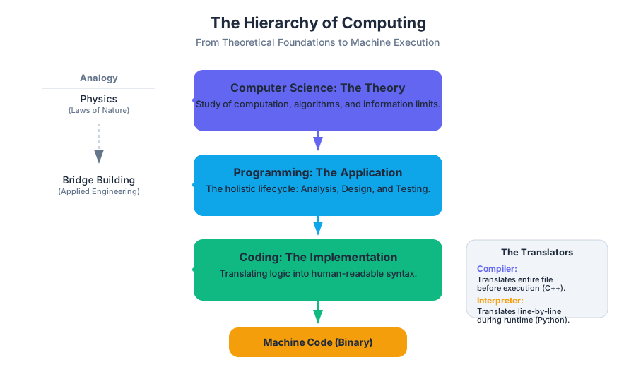
To understand the relationship between Computer Science (CS) and programming, one might look to the relationship between physics and bridge building. Physics provides the fundamental laws of motion, gravity, and material stress; bridge building is the application of those laws to solve a specific problem.
Computer Science: The Theoretical Foundation
Computer Science is a branch of mathematics and engineering that focuses on the theory of computation. It asks fundamental questions: What can be computed? How much time and memory will it take? How can we represent complex data structures efficiently?
Definition: Computer Science is the study of the storage, transformation, and transfer of information. It encompasses the design of algorithms, the architecture of hardware, and the limits of what machines can achieve.
Programming: The Applied Craft
Programming is the act of instructing a computer to perform specific tasks. It is the implementation phase of computer science. A programmer uses the principles discovered by computer scientists to build applications, websites, and systems.
| Feature | Computer Science | Programming |
|---|---|---|
| Primary Goal | Understanding the limits and possibilities of computation. | Solving specific problems and building functional software. |
| Core Activity | Developing proofs, analyzing complexity ($O(n)$), and designing architectures. | Writing code, debugging, and maintaining systems. |
| Key Question | "Is this problem solvable, and what is the most efficient way?" | "How do I implement this feature and ensure it works for the user?" |
| Output | Algorithms, theorems, and architectural patterns. | Executable applications, scripts, and libraries. |
Coding vs. Programming
In modern discourse, the terms coding and programming are frequently used as synonyms. However, in a professional and academic context, they represent different levels of the software development lifecycle.
Coding: The Translation Layer
Coding is the process of translating a set of logic or a specific algorithm into a syntax that a computer can execute. It is a subset of programming. If programming is "writing a novel," coding is the act of "typing the sentences."
Programming: The Holistic Lifecycle
Programming involves a much broader scope. It includes:
- Problem Analysis: Understanding the requirements.
- Algorithm Design: Planning the logic before a single line is written.
- Coding: The actual implementation in a language like Python or C.
- Testing and Debugging: Ensuring the logic holds up under edge cases.
- Maintenance: Updating the code as requirements change.
Low-Level Implementation Example
To illustrate the difference, consider the task of managing memory—a core concern in systems programming. A "coder" might follow a pattern, but a "programmer" understands the underlying memory map.
/*
 * A low-level C implementation of a dynamic array (vector).
 * This demonstrates the "Programming" aspect: managing
 * heap memory, pointers, and growth strategies.
 */

#include <stdio.h>
#include <stdlib.h>

typedef struct {
    int *data;
    size_t size;
    size_t capacity;
} IntVector;

void init_vector(IntVector *v, size_t initial_capacity) {
    v->data = (int *)malloc(initial_capacity * sizeof(int));
    v->size = 0;
    v->capacity = initial_capacity;
}

void push_back(IntVector *v, int value) {
    if (v->size == v->capacity) {
        // Geometric expansion: doubling capacity to achieve O(1) amortized time
        v->capacity *= 2;
        v->data = (int *)realloc(v->data, v->capacity * sizeof(int));
    }
    v->data[v->size++] = value;
}

int main() {
    IntVector myVec;
    init_vector(&myVec, 2);
    push_back(&myVec, 10);
    push_back(&myVec, 20);
    push_back(&myVec, 30); // Triggers realloc

    printf("Vector size: %zu, Capacity: %zu\n", myVec.size, myVec.capacity);
    free(myVec.data);
    return 0;
}
Compilers and Interpreters
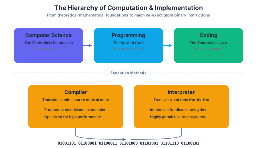
Computers do not "understand" Python, Java, or C++. The Central Processing Unit (CPU) only executes Machine Code—a series of binary instructions (1s and 0s) that correspond to physical logic gates. To bridge the gap between human-readable code and machine-executable instructions, we use translators: Compilers and Interpreters.
The Compiler
A Compiler translates the entire source code into a standalone machine-code file (an executable) before the program runs.
- Lexical Analysis: Breaking code into "tokens."
- Parsing: Building an Abstract Syntax Tree (AST) to check for grammatical errors.
- Optimization: Reorganizing logic to run faster.
- Code Generation: Producing the binary file.
The Interpreter
An Interpreter translates and executes the code line-by-line (or block-by-block) at runtime. Python is primarily an interpreted language.
| Feature | Compiler | Interpreter |
|---|---|---|
| Execution | Translates once, runs many times. | Translates and runs simultaneously. |
| Speed | Faster execution (pre-optimized). | Slower execution (translation overhead). |
| Feedback | Errors reported after the whole file is scanned. | Errors reported the moment the line is reached. |
| Portability | Target-specific (e.g., Windows .exe won't run on Mac). | Highly portable (runs anywhere the interpreter is installed). |
Mathematical Derivation of Execution Time
The total time $T$ to run a program can be modeled differently for both systems.
For a Compiler: $$T_{total} = T_{compile} + T_{execute}$$ Since $T_{compile}$ happens only once, for $N$ executions, the average time per run is: $$\frac{T_{compile} + N \cdot T_{execute}}{N} \approx T_{execute} \text{ (as } N \to \infty)$$
For an Interpreter: $$T_{total} = N \cdot (T_{translate_line} + T_{execute_line})$$ The translation overhead is incurred every single time the program runs.
# Pseudocode: The Logic of a Simple Interpreter Loop
# --------------------------------------------------
WHILE program_counter < length_of_source:
    line = fetch_next_line(source_code)
    tokens = tokenize(line)
    syntax_tree = parse(tokens)

    IF syntax_tree.is_valid():
        result = execute_immediate(syntax_tree)
        update_environment_state(result)
    ELSE:
        throw_syntax_error(line_number)
        BREAK
Python: Libraries and Applications
Python has emerged as the premier language for introductory computer science and professional data science due to its "batteries included" philosophy. This refers to the Standard Library and the vast ecosystem of third-party packages.
What is a Library?
A Library is a collection of pre-written code that programmers can use to optimize their workflow. Instead of writing a complex mathematical function from scratch, you "import" a library that has already been tested and optimized by experts.
Major Python Application Domains
Python’s versatility is driven by specific libraries that dominate various industries:
| Domain | Key Libraries | Description |
|---|---|---|
| Data Science | NumPy, Pandas | High-performance array processing and data manipulation. |
| Machine Learning | PyTorch, TensorFlow | Building and training neural networks. |
| Web Development | Django, Flask | Backend frameworks for building scalable websites. |
| Automation | Selenium, BeautifulSoup | Web scraping and browser automation. |
| Scientific Computing | SciPy, Matplotlib | Advanced calculus, signal processing, and 2D/3D visualization. |
Real-World Usage: Data Analysis
The following example demonstrates how a library like pandas abstracts away hundreds of lines of manual file-parsing and calculation logic.
import pandas as pd
import matplotlib.pyplot as plt

# Realistic usage: Analyzing a CSV of global temperatures
def analyze_climate_data(file_path):
    # Load data into a DataFrame (Abstraction of file I/O)
    df = pd.read_csv(file_path)

    # Perform complex filtering and aggregation in two lines
    df['Year'] = pd.to_datetime(df['Date']).dt.year
    yearly_avg = df.groupby('Year')['Temperature'].mean()

    # Visualization (Abstraction of graphics rendering)
    plt.figure(figsize=(10, 5))
    plt.plot(yearly_avg.index, yearly_avg.values, label='Avg Global Temp')
    plt.title("Climate Trends Over Time")
    plt.xlabel("Year")
    plt.ylabel("Temperature (Celsius)")
    plt.legend()
    plt.show()

# Execution would look like:
# analyze_climate_data('global_temps.csv')
Computational Thinking: The Core of the Discipline
Beyond syntax and tools, the most critical skill in Computer Science is Computational Thinking. This is a problem-solving process that involves breaking down complex problems into manageable parts that a computer can solve.
The Four Pillars of Computational Thinking
- Decomposition: Breaking a large problem into smaller, logical sub-problems. (e.g., breaking "Build a Game" into "Player Movement," "Enemy AI," and "Score Tracking").
- Pattern Recognition: Identifying similarities or trends within a problem.
- Abstraction: Focusing on the important information while ignoring irrelevant details.
- Algorithms: Developing a step-by-step solution to the problem.
Worked Example: The Accumulator Pattern
Suppose we want to calculate the sum of all even numbers in a list. This requires an algorithmic approach:
- Initialize a variable
totalto 0 (State). - Look at each number in the list (Iteration).
- Check if the number is divisible by 2 (Conditional Logic).
- If yes, add it to
total(Mutation).
# Example of executing a Python script from the command line
# This shows how the interpreter is invoked in a real environment.

$ python3 --version
Python 3.10.12

$ cat sum_evens.py
numbers = [1, 2, 3, 4, 5, 6, 7, 8, 9, 10]
total = sum(n for n in numbers if n % 2 == 0)
print(f"The sum of evens is: {total}")

$ python3 sum_evens.py
The sum of evens is: 30
Common Pitfalls and Misconceptions
As students transition from "using" technology to "creating" it, several common hurdles emerge:
- The "Magic" Fallacy: Believing the computer "knows" what you mean. Computers are literal. If you have a typo in a variable name, the computer doesn't see a "small mistake"; it sees a completely different entity.
- Syntax vs. Logic: Beginners often spend 90% of their time worrying about where the colons and parentheses go (syntax). However, the most difficult bugs are logical errors, where the code runs perfectly but produces the wrong answer because the algorithm is flawed.
- Python is "Easy": While Python's syntax is readable, the computer science concepts it implements (like Object-Oriented Programming or Recursion) are just as rigorous as in any other language.
Key Insight: Learning to program is not about memorizing commands; it is about learning to think in a way that is structured, logical, and exhaustive.
Technical Requirements and the Development Environment
Key concepts: JavaScript requirements · Integrated Development Environment (IDE) · Code Editor · Console and Output
Covers the essential browser settings and the integrated development environment (IDE) used throughout the course.
Technical Requirements and the Development Environment
The transition from a passive consumer of technology to an active creator begins with the establishment of a robust Development Environment. In the context of modern computer science education—specifically within the Khan Academy "Client Challenge" framework—this environment is not merely a text box, but a sophisticated, browser-based Integrated Development Environment (IDE). Understanding the technical prerequisites and the internal mechanics of this environment is essential for minimizing "environmental friction," allowing the programmer to focus entirely on algorithmic logic and computational thinking.
The JavaScript Prerequisite: The Engine of Interactivity
The primary technical requirement for modern web-based programming is the activation of JavaScript within the client's browser. While the learner is writing Python code, the platform itself—the editor, the real-time error checker, and the output console—is constructed using a complex stack of JavaScript frameworks.
Why JavaScript Matters
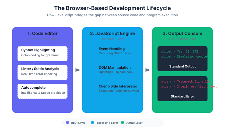
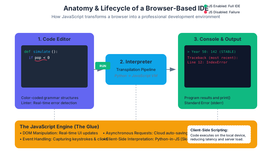
JavaScript serves as the "glue" between the user's input and the server's response. In a browser-based IDE, JavaScript handles:
- DOM Manipulation: Updating the interface dynamically as the user types.
- Event Handling: Capturing keystrokes, mouse clicks on the "Run" button, and scroll events.
- Asynchronous Requests: Saving code progress to the cloud without refreshing the page.
- Client-Side Interpretation: Many modern platforms use JavaScript-based interpreters (like Skulpt or Pyodide) to run Python code directly in the browser, reducing latency and server load.
Definition: Client-Side Scripting Client-side scripting refers to the execution of scripts, such as JavaScript, on the user's local device rather than on the web server. This allows for immediate feedback and highly interactive user interfaces, which are critical for coding environments.
| Requirement State | Impact on IDE Functionality | User Experience |
|---|---|---|
| JavaScript Enabled | Full access to editor, console, and interactive simulations. | Fluid, real-time feedback and code execution. |
| JavaScript Disabled | Total failure of the IDE interface; "Client Challenge" guide inaccessible. | Static error message: "Please enable JavaScript to proceed." |
| Partial Block (NoScript) | Broken UI elements; syntax highlighting may fail; "Run" button unresponsive. | Frustrating, intermittent failures and data loss. |
Anatomy of the Integrated Development Environment (IDE)
An Integrated Development Environment (IDE) is a software suite that consolidates the basic tools required to write and test software. For the beginner, the IDE simplifies the complex toolchain of compilers, linkers, and debuggers into a unified interface.
The Code Editor: The Interface of Logic
The Code Editor is a specialized text editor designed for writing source code. Unlike a standard word processor, it treats text as a structured hierarchy of instructions.
- Syntax Highlighting: The editor parses the code in real-time and applies color-coding based on the language's grammar. For example, Python keywords like
if,while, anddefappear in one color, while strings and integers appear in others. This reduces cognitive load by allowing the brain to recognize patterns quickly. - Linters and Static Analysis: As you type, the editor performs "background checks." If you forget a colon at the end of a
forloop, a red underline (often called a "squiggle") appears. This is the linter identifying a syntax error before the code is even executed. - Autocomplete (IntelliSense): The editor predicts the variable or function name you are typing based on the current Scope and the libraries imported.
The Console and Output
The Console is the terminal window where the program "speaks" back to the user. It serves two primary roles:
- Standard Output (stdout): Displays text generated by
print()statements. - Standard Error (stderr): Displays Tracebacks—detailed reports of why a program crashed, including the line number and the type of error (e.g.,
IndexError,TypeError).
Implementation: The Execution Lifecycle
When a user clicks the Run Button, a multi-stage pipeline is triggered. In a browser-based Python environment, this often involves transpilation or a virtual machine (VM) implementation.
First Code Block: Low-Level Logic Simulation
The following Python code demonstrates a non-trivial simulation of a population dynamic, a common pattern in the "Client Challenge" curriculum. It utilizes loops, conditional logic, and state mutation.
import random

def simulate_population(initial_pop, growth_rate, years, catastrophe_chance):
    """
    Simulates population growth with stochastic interference.
    Demonstrates state management and loop control flow.
    """
    current_pop = initial_pop
    history = []

    for year in range(1, years + 1):
        # Calculate growth
        births = int(current_pop * growth_rate)
        current_pop += births

        # Stochastic event: Catastrophe
        if random.random() < catastrophe_chance:
            loss = int(current_pop * 0.5)
            current_pop -= loss
            event = "CATASTROPHE"
        else:
            event = "STABLE"

        history.append({
            "year": year,
            "population": current_pop,
            "status": event
        })

        # Exit condition: Extinction
        if current_pop <= 0:
            print(f"Extinction reached at year {year}")
            break

    return history

# Execution call
results = simulate_population(100, 0.1, 50, 0.05)
for entry in results[-5:]: # View last 5 years
    print(f"Year {entry['year']}: {entry['population']} ({entry['status']})")
Second Code Block: Algorithmic Derivation (Pseudocode)
To understand what the IDE is doing behind the scenes, we can look at the Loop Design Pattern used in the simulation above.
ALGORITHM: StochasticPopulationGrowth
INPUT: P (initial), r (rate), t (time), c (catastrophe probability)
OUTPUT: List of population states

BEGIN
    SET current_P = P
    CREATE empty list HISTORY

    FOR each year from 1 to t:
        COMPUTE births = current_P * r
        INCREMENT current_P BY births

        GENERATE random_val between 0 and 1
        IF random_val < c THEN:
            DECREMENT current_P BY (current_P * 0.5)
            SET status = "CATASTROPHE"
        ELSE:
            SET status = "STABLE"
        ENDIF

        APPEND {year, current_P, status} TO HISTORY

        IF current_P <= 0 THEN:
            EXIT LOOP
        ENDIF
    ENDFOR

    RETURN HISTORY
END
IDE Component Comparison
Programmers often choose their environment based on the balance between "weight" (resource usage) and "features."
| Feature | Browser-Based IDE (Khan Academy) | Local IDE (VS Code / PyCharm) | Professional Command Line (Vim/Tmux) |
|---|---|---|---|
| Setup Complexity | Zero (Requires only a browser) | Moderate (Requires Python install) | High (Requires config files) |
| Execution Context | Sandboxed (Safe, limited access) | Local System (Full file access) | Local/Remote Server |
| Collaboration | High (Spin-offs, shared URLs) | Moderate (Git integration) | High (SSH/Shared servers) |
| Offline Access | No | Yes | Yes |
Advanced Concepts: State, Scope, and Debugging
The development environment is responsible for tracking the State of the program—the current value of all variables at a specific moment in time.
Computational Thinking: Sequence and State
Computers execute instructions in a Sequence. However, the outcome of an instruction often depends on the current State.
- Variables act as containers for state.
- Type Casting (e.g., converting a string
"10"to an integer10) is a common requirement when handling user input from the console.
Debugging and the "Mental Model"
Debugging is the process of reconciling the computer's actual behavior with the programmer's Mental Model. The IDE assists this through:
- Breakpoints: Pausing execution at a specific line to inspect variables.
- Step-through: Executing code one line at a time.
- Watch Expressions: Monitoring a specific variable's value as it changes across loops.
The Golden Rule of Debugging If the output is not what you expected, your mental model of the state is incorrect. Use
print()statements or the IDE's debugger to expose the "hidden" state of the machine.
Third Code Block: Environment Configuration (JSON)
In professional environments, the IDE itself is configured via code. Below is a representation of how an IDE's settings.json might define the Python environment and linter rules.
{
    "python.pythonPath": "/usr/local/bin/python3",
    "editor.fontSize": 14,
    "editor.formatOnSave": true,
    "python.linting.enabled": true,
    "python.linting.pylintEnabled": true,
    "editor.tokenColorCustomizations": {
        "comments": "#608b4e",
        "functions": "#dcdcaa",
        "keywords": "#569cd6"
    },
    "terminal.integrated.shell.osx": "/bin/zsh"
}
The "Spin-off" Mechanism: Collaborative Development
A unique feature of the Khan Academy development environment is the Spin-off. This is a functional implementation of Forking in version control.
- Original Project: The "Master" version of a challenge or project.
- Spin-off: A personal copy saved to the learner's profile.
- Persistence: Changes made in a spin-off do not affect the original, allowing for "sandbox" experimentation.
This mirrors professional workflows where developers "fork" a repository on GitHub to propose changes or build new features without risking the stability of the main codebase.
Common Pitfalls in the Development Environment
Even with a powerful IDE, learners frequently encounter specific "environmental" hurdles:
- Indentation Errors: Python uses whitespace to define scope. A single space or tab out of alignment will cause a
IndentationError. Modern IDEs help by showing "indentation guides" (vertical lines). - Global vs. Local Scope: Defining a variable inside a function (Local) and trying to access it outside (Global) is a common source of
NameError. - Infinite Loops: A
whileloop without a proper exit condition will hang the browser. The IDE usually has a "timeout" mechanism to kill scripts that run for too long. - Case Sensitivity: Python treats
myVariableandmyvariableas two completely different entities.
| Error Type | Cause | IDE Feedback |
|---|---|---|
| Syntax Error | Violating the rules of the language (e.g., missing parenthesis). | Red underlines; program won't start. |
| Runtime Error | Valid code that tries to do something impossible (e.g., divide by zero). | Traceback in the console during execution. |
| Logical Error | Code runs perfectly but produces the wrong result. | No error message; requires manual debugging. |
Summary of Technical Workflow
The journey from a blank file to a working program follows a predictable pipeline within the IDE:
- Initialization: Ensure JavaScript is enabled and the environment loads.
- Drafting: Write code in the editor, utilizing syntax highlighting and autocomplete.
- Static Analysis: Address any linter warnings or syntax errors highlighted by the IDE.
- Execution: Click "Run" to pass the code to the interpreter.
- Observation: Analyze the output in the console.
- Iteration: If a runtime or logical error occurs, modify the code and repeat from step 4.
- Persistence: Save the work as a "Spin-off" for future refinement.
Conclusion: The IDE as a Force Multiplier
The development environment is more than a tool; it is a partner in the creative process. By automating the mundane aspects of programming—such as checking for typos, managing file paths, and formatting text—the IDE allows the programmer to operate at a higher level of abstraction. Whether you are building a simple "Hello World" or a complex population simulation, mastering your environment is the first step toward mastering the machine.
Unit 1: Computational Thinking and Variables
Key concepts: Computational thinking (sequence and state) · Data types (Integers, Floats, Booleans, Strings) · Variables · Binary Data
Introduces the basics of how computers interpret sequence and state using data types and variables.
Unit 1: Computational Thinking and Variables
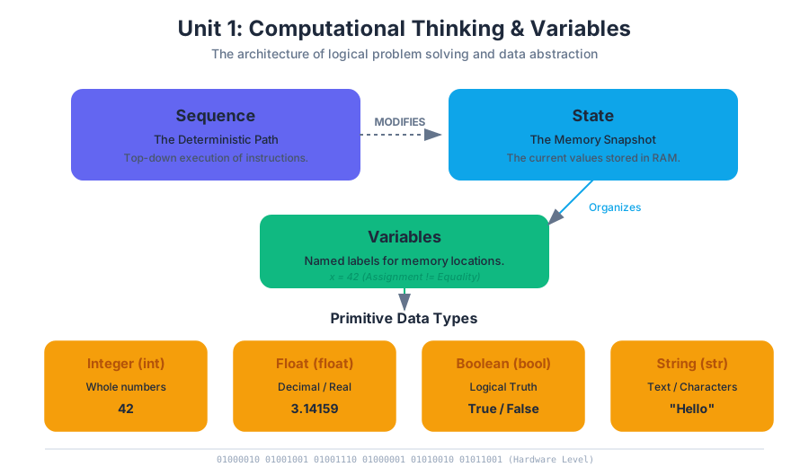
Computational thinking is the foundational cognitive process of formulating a problem and expressing its solution in such a way that a computer—a purely logical, state-driven machine—can effectively carry it out. While often conflated with "learning to code," computational thinking is a broader analytical framework. It involves breaking down complex systems into discrete components, identifying patterns, and abstracting away unnecessary details to create a repeatable sequence of instructions.
In this unit, we explore the dual pillars of digital computation: Sequence and State. We will examine how human-readable information is distilled into binary data, how that data is categorized into primitive types, and how variables serve as the fundamental mechanism for managing information over time.
1.1 The Mechanics of Computational Thinking: Sequence and State
At its core, every computer program is a manipulation of state through a defined sequence of operations. To think computationally is to view the world through these two lenses.
1.1.1 Sequence: The Deterministic Path
A sequence is the specific order in which instructions are executed. Computers are inherently "top-down" processors; they do not possess intuition and cannot skip steps unless explicitly told to do so. A change in the sequence of even a single line of code can fundamentally alter the outcome of a program.
The Principle of Sequentiality: In a synchronous execution environment, instruction $I_{n+1}$ cannot begin until instruction $I_n$ has completed its transformation of the system state.
1.1.2 State: The Snapshot of Memory
State refers to the condition of a system at a specific point in time. In programming, the state is the sum total of all stored values in the computer's memory (RAM). As a program executes its sequence, it modifies the state.
| Concept | Definition | Real-World Analogy |
|---|---|---|
| Sequence | The ordered set of instructions. | A recipe's step-by-step instructions. |
| State | The current values of all variables. | The current temperature and ingredients in the bowl. |
| Transition | The act of moving from one state to another. | The act of mixing the ingredients. |
1.1.3 Why it Matters
Understanding state and sequence is critical for debugging. Most logical errors (bugs) arise because the programmer has an incorrect mental model of the state at a specific step in the sequence. By tracing the state through the sequence, developers can pinpoint exactly where the logic diverges from the intended outcome.
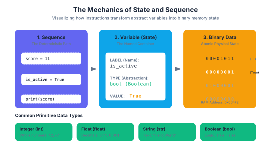
1.2 Binary Data: The Atomic Level of Information
Before we can discuss variables, we must understand the medium they inhabit. Computers do not "know" what a number or a letter is. They operate on physical voltages that we interpret as Binary Data.
1.2.1 Bits, Bytes, and Bases
The fundamental unit of information is the bit (binary digit), representing a choice between two mutually exclusive states: 0 (Off/False) and 1 (On/True).
- Bit: A single 0 or 1.
- Byte: A group of 8 bits. A byte can represent $2^8$ (256) distinct values.
- Word: The natural unit of data used by a particular processor design (typically 32 or 64 bits in modern systems).
1.2.2 The Binary-to-Decimal Derivation
To represent a decimal number in binary, we use a positional notation system where each place value is a power of 2.
$$Value = \sum_{i=0}^{n-1} d_i \times 2^i$$
Where $d$ is the digit (0 or 1) at position $i$.
Example: Converting 1011 to Decimal
- $(1 \times 2^3) = 8$
- $(0 \times 2^2) = 0$
- $(1 \times 2^1) = 2$
- $(1 \times 2^0) = 1$
- Total: $8 + 0 + 2 + 1 = 11$
1.3 Primitive Data Types
While everything is binary at the hardware level, high-level languages like Python provide Data Types—abstractions that tell the computer how to interpret a specific sequence of bits and what operations are valid on that data.
1.3.1 Integers (int)
Integers are whole numbers without a fractional component. In many languages (like C or Java), integers have a fixed size (e.g., 32-bit). Python, however, uses "arbitrary-precision integers," meaning they can grow as large as the available memory allows.
1.3.2 Floating-Point Numbers (float)
Floats represent real numbers (decimals). They follow the IEEE 754 standard, which stores numbers in scientific notation: $Sign \times Fraction \times 2^{Exponent}$.
The Floating-Point Pitfall: Because floats are approximations of real numbers in base-2, some decimal fractions (like 0.1) cannot be represented exactly. This leads to precision errors in long calculations.
1.3.3 Booleans (bool)
Named after George Boole, the Boolean type represents logical truth values: True or False. In memory, these are often stored as a single byte (00000001 for True, 00000000 for False).
1.3.4 Strings (str)
Strings are sequences of characters. To store text, the computer uses an encoding standard like ASCII or UTF-8 to map numbers to symbols. For example, the letter 'A' is mapped to the decimal value 65 (binary 01000001).
| Data Type | Python Keyword | Example | Typical Size |
|---|---|---|---|
| Integer | int |
42 |
Variable (Python) / 4-8 bytes (C) |
| Float | float |
3.14159 |
8 bytes (64-bit) |
| Boolean | bool |
True |
1 byte |
| String | str |
"Hello" |
1 byte per ASCII char + overhead |
1.4 Variables: Naming the State
A variable is a reserved location in the computer's memory used to store a value. It acts as a "label" or "container" for data, allowing the programmer to refer to a value by name rather than by its memory address.
1.4.1 Assignment and Memory
In Python, the assignment operator = does not mean "mathematical equality." It means "evaluate the expression on the right and bind the result to the name on the left."
# Python Implementation: Demonstrating State and Type Dynamics
current_user_count = 150  # Integer assignment
growth_rate = 1.05        # Float assignment
is_active = True          # Boolean assignment
system_msg = "Status: OK" # String assignment

# State Transition
# The right side is evaluated first (150 * 1.05 = 157.5)
# Then the name 'current_user_count' is rebound to the new float value.
current_user_count = current_user_count * growth_rate

print(f"{system_msg} | Users: {current_user_count} | Active: {is_active}")
1.4.2 Low-Level Perspective
In lower-level languages like C, we must declare the type explicitly, which tells the compiler exactly how many bytes to allocate on the "stack."
/* C Implementation: Explicit Memory Allocation */
#include <stdio.h>
#include <stdbool.h>

int main() {
    int age = 25;           // Allocates 4 bytes
    double pi = 3.14159;    // Allocates 8 bytes
    bool is_valid = true;   // Allocates 1 byte

    // Printing memory addresses to show where the 'state' lives
    printf("Value: %d, Address: %p\n", age, (void*)&age);
    return 0;
}
1.4.3 Variable Naming Conventions
To maintain readability and prevent syntax errors, variables must follow specific rules:
- Must start with a letter or underscore (
_). - Cannot start with a number.
- Can only contain alphanumeric characters and underscores (
A-z,0-9,_). - Case-sensitive (
Ageandageare different variables). - Avoid Reserved Keywords: Do not name variables
if,while,class, orTrue.
1.5 Arithmetic Operators and Type Casting
Computers perform operations based on the data types involved. This is known as Operator Overloading. For example, the + operator adds two integers but concatenates (joins) two strings.
1.5.1 Standard Operators
| Operator | Name | Description | Example (x=10, y=3) |
|---|---|---|---|
+ |
Addition | Sum of values | 13 |
- |
Subtraction | Difference | 7 |
* |
Multiplication | Product | 30 |
/ |
Division | Quotient (always returns a float) | 3.333... |
// |
Floor Division | Quotient without remainder | 3 |
% |
Modulo | Remainder of division | 1 |
** |
Exponentiation | Power of | 1000 |
1.5.2 Type Casting (Conversion)
Sometimes we need to convert data from one type to another. This is called Type Casting.
- Implicit Casting: Python automatically converts an integer to a float during division.
- Explicit Casting: The programmer manually converts a type using functions like
int(),float(), orstr().
\text{Algorithm: Input Normalization}
\begin{enumerate}
    \item \text{Receive input } S \text{ as a String.}
    \item \text{Attempt conversion: } N = \text{float}(S)
    \item \text{If } N < 0, \text{ set } State = \text{"Error"}
    \item \text{Else, calculate } Result = N \times \text{Constant}
\end{enumerate}
1.6 Common Pitfalls and Best Practices
1.6.1 The "Off-by-One" and Precision Errors
Beginners often assume 0.1 + 0.2 == 0.3 will evaluate to True. In reality, due to binary float representation, it evaluates to False (the result is actually 0.30000000000000004).
Solution: When comparing floats, check if the difference is smaller than a tiny threshold (epsilon): abs(a - b) < 0.00001.
1.6.2 Uninitialized Variables
Attempting to use a variable before assigning it a value will result in a NameError. The "state" of that name does not exist yet in the program's namespace.
1.6.3 Type Mismatch
Trying to add a string and an integer (e.g., "Age: " + 25) will cause a TypeError. You must explicitly cast the integer to a string: "Age: " + str(25).
1.7 Summary of the Computational Pipeline
- Input: Data enters the system (often as strings from a keyboard or file).
- Casting: Data is converted into appropriate types (Integers for counts, Floats for measurements).
- Processing: The Sequence of instructions modifies the State using arithmetic and logic.
- Output: The final state is converted back into a human-readable format (Strings) and displayed.
Further Exploration: The Von Neumann Architecture
To truly master Unit 1, one should investigate the Von Neumann Architecture, which describes the physical hardware implementation of sequence and state. It consists of a Central Processing Unit (CPU) that fetches instructions in sequence and a Memory Unit that stores the program's state. This hardware reality is what necessitates the software concepts of variables and data types we have explored here.
Unit 1: Expressions, Operators, and Output
Key concepts: Arithmetic operators · String Concatenation · The print() Function · Type casting · Program Execution Tracing
Explains how Python manipulates data using operators and displays results via the print function.
Unit 1: Expressions, Operators, and Output
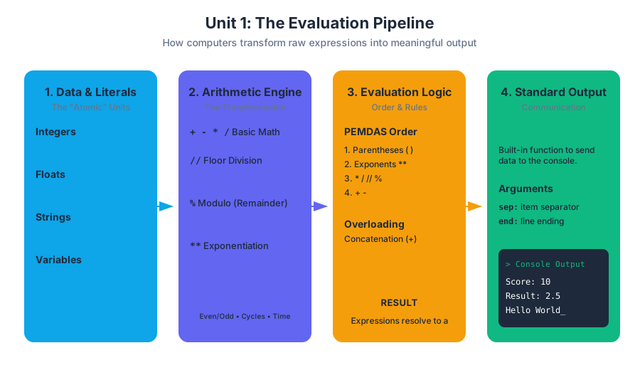
In the study of Computer Science, we begin not with complex algorithms or artificial intelligence, but with the "atomic" units of computation: Expressions and Output. At its core, every program you will ever write is a mechanism for transforming data from one state to another and communicating that state to the outside world. This unit establishes the foundational mental model required to understand how a computer evaluates logic, manages data types, and executes instructions in a linear sequence.
The Nature of Computation: State and Logic
Before diving into syntax, one must understand that a computer is essentially a high-speed calculator with a memory. Computation is the process of taking input, applying a series of expressions to it, and producing an output.
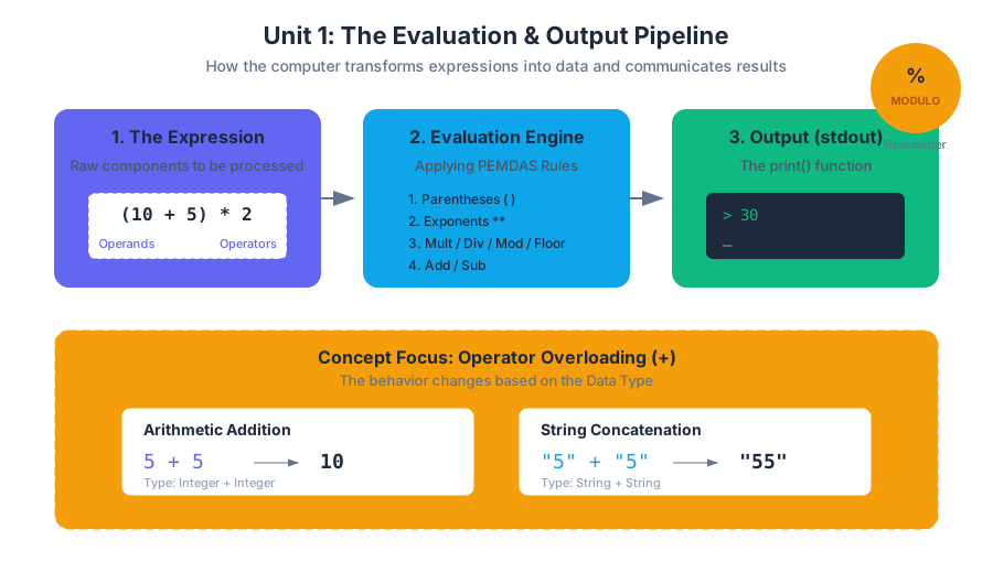
Definition: Expression An expression is a combination of values, variables, and operators that the Python interpreter evaluates to produce a single value. For example,
2 + 3is an expression that evaluates to the value5.
The process of "simplifying" an expression is called evaluation. Unlike human language, which can be ambiguous, programming expressions follow strict mathematical rules. If an expression is syntactically correct, it will always resolve to a single, predictable result.
Arithmetic Operators and Precedence
Arithmetic operators are the symbols that tell the computer which mathematical operation to perform. While most are familiar from basic algebra, their behavior in a programming environment involves nuances regarding data types and "order of operations."
The Primary Operators
Python supports the standard suite of arithmetic operators, categorized by their function:
| Operator | Name | Description | Example | Result |
|---|---|---|---|---|
+ |
Addition | Adds two operands | 10 + 5 |
15 |
- |
Subtraction | Subtracts the right operand from the left | 10 - 5 |
5 |
* |
Multiplication | Multiplies two operands | 10 * 5 |
50 |
/ |
Division | Divides left operand by right (always returns a float) | 10 / 4 |
2.5 |
// |
Floor Division | Divides and rounds down to the nearest integer | 10 // 4 |
2 |
% |
Modulo | Returns the remainder of the division | 10 % 3 |
1 |
** |
Exponentiation | Raises the left operand to the power of the right | 2 ** 3 |
8 |
The Modulo Operator (%)
The Modulo operator is often the most confusing for beginners but is arguably one of the most useful in computer science. It returns the remainder of a division operation.
- Parity Checking:
x % 2 == 0determines if a number is even. - Cyclic Sequences: In a game with 4 players,
turn % 4ensures the turn counter always stays within the range 0–3. - Time Calculations:
total_seconds % 60gives you the remaining seconds after extracting whole minutes.
Operator Precedence (PEMDAS)
Computers do not read expressions from left to right in a simple sweep. They follow Operator Precedence, which dictates the order in which parts of an expression are evaluated.
- Parentheses
() - Exponentiation
** - Multiplication, Division, Floor Division, Modulo
*,/,//,%(evaluated left-to-right) - Addition, Subtraction
+,-(evaluated left-to-right)
/*
   Low-level implementation perspective:
   In C, we must be wary of integer overflow and the distinction
   between types during arithmetic. This snippet demonstrates
   how a simple modulo-based parity check looks in a systems context.
*/

#include <stdio.h>

int main() {
    int numerator = 17;
    int denominator = 5;

    // Integer division truncates decimals
    int quotient = numerator / denominator;
    // Modulo finds the remainder
    int remainder = numerator % denominator;

    printf("Quotient: %d, Remainder: %d\n", quotient, remainder);

    // Bitwise check for parity (more efficient than modulo at CPU level)
    if ((numerator & 1) == 0) {
        printf("%d is Even\n", numerator);
    } else {
        printf("%d is Odd\n", numerator);
    }

    return 0;
}
String Concatenation: The + Operator Overloaded
In programming, operator overloading occurs when a single symbol has different behaviors depending on the data types (operands) involved. The + symbol is the primary example:
- With Integers/Floats: It performs mathematical addition.
- With Strings: It performs concatenation, which is the process of joining two strings end-to-end.
Formal Definition of Concatenation
Mathematically, if we have two strings $S_1$ and $S_2$ from an alphabet $\Sigma$, the concatenation $S_1 \cdot S_2$ results in a new string containing the characters of $S_1$ followed by $S_2$.
\text{Let } S_1 = \text{"Hello"}, S_2 = \text{"World"}
\\
S_1 + S_2 = \text{"HelloWorld"}
\\
\text{Note: Concatenation is not commutative: } S_1 + S_2 \neq S_2 + S_1
Common Pitfalls in Concatenation
A frequent error is attempting to concatenate a string with a numeric type without conversion.
"Score: " + 10$\rightarrow$ TypeError: can only concatenate str (not "int") to str."5" + "5"$\rightarrow$"55"(String concatenation).5 + 5$\rightarrow$10(Mathematical addition).
The print() Function: Communicating with the User
The print() function is the standard method for sending data to the Console (or stdout). It is a built-in function that takes one or more arguments, converts them to strings, and displays them.
Anatomy of a Print Call
The print() function is more powerful than it appears. It includes optional keyword arguments that control its behavior:
sep: The string inserted between multiple values (default is a space).end: The string printed at the very end of the call (default is a newline\n).
# Realistic usage: Formatting output for a data report
username = "Admin_Alpha"
login_attempts = 3
success_rate = 92.5

# Using f-strings (formatted string literals) for clean output
print(f"--- USER REPORT: {username} ---")
print("Status:", "Active", "Verified", sep=" | ")
print("Attempts:", login_attempts, end=" --> ")
print(f"Success: {success_rate}%")

# Output:
# --- USER REPORT: Admin_Alpha ---
# Status: Active | Verified
# Attempts: 3 --> Success: 92.5%
Type Casting: Changing the "Shape" of Data
Data in Python is strongly typed, meaning the interpreter cares deeply about what "kind" of data a value is. However, Python is also dynamically typed, meaning variables can change types over time. Type Casting is the explicit process of converting a value from one data type to another.
Why Cast?
The most common reason for casting is handling User Input. In Python, the input() function always returns a string. If you ask a user for their age, you receive "25", not 25. To perform math on that age, you must cast it.
Conversion Table
| Target Type | Function | Input Example | Output Example | Note |
|---|---|---|---|---|
| Integer | int() |
"10" |
10 |
Drops decimals if converting from float. |
| Float | float() |
10 |
10.0 |
Adds .0 to integers. |
| String | str() |
100 |
"100" |
Essential for concatenation. |
| Boolean | bool() |
1 |
True |
0, None, and empty strings return False. |
Explicit vs. Implicit Casting
- Implicit (Coercion): Python does this automatically. If you add an
intto afloat(5 + 2.0), Python promotes the integer to a float to avoid losing precision, resulting in7.0. - Explicit: The programmer manually uses functions like
int()orstr().
# Shell script analogy: Type handling in Bash is much looser than Python.
# Everything is essentially a string, and we use 'bc' or '(( ))' for math.

VAR1="10"
VAR2="20"

# String concatenation in Bash
COMBINED="$VAR1$VAR2"
echo "Concatenated: $COMBINED" # Result: 1020

# Arithmetic evaluation (Explicit casting to integer context)
SUM=$((VAR1 + VAR2))
echo "Sum: $SUM" # Result: 30
Program Execution Tracing
Tracing is the mental or physical process of stepping through code line-by-line to track the state of variables and the flow of execution. This is the single most important skill for debugging.
The Trace Table
A trace table tracks the value of every variable after each line of code is executed. Consider the following code:
x = 10
y = 5
x = x + y
y = x * 2
print(x + y)
Step-by-Step Trace
| Line # | Instruction | x value |
y value |
Output |
|---|---|---|---|---|
| 1 | x = 10 |
10 | undefined | - |
| 2 | y = 5 |
10 | 5 | - |
| 3 | x = x + y |
15 | 5 | - |
| 4 | y = x * 2 |
15 | 30 | - |
| 5 | print(x + y) |
15 | 30 | 45 |
The "Mental Model" of the Interpreter
When tracing, you must act as the interpreter. This means:
- Evaluate the right side of an assignment (
=) completely before changing the variable on the left. - Update the State: Once a variable is updated, its old value is gone forever (unless stored elsewhere).
- Sequential Flow: Execution always moves from top to bottom unless a control structure (like a loop or function) redirects it.
Common Pitfalls and Edge Cases
1. Floating Point Imprecision
Computers represent decimal numbers in binary, which can lead to tiny errors in precision.
0.1 + 0.2in Python results in0.30000000000000004.- Lesson: Never use
==to compare two floats; instead, check if the difference between them is very small.
2. Division by Zero
Attempting to divide by zero (using /, //, or %) will trigger a ZeroDivisionError. This is a "runtime error" that crashes the program.
3. String Multiplication
While you cannot add a string and an integer, you can multiply them.
"Echo" * 3results in"EchoEchoEcho".- This is a unique Python feature used for creating visual separators in console apps.
4. The "Input is String" Trap
age = input("Enter age: ")
print(age + 1) # CRASH! age is a string.
Always wrap numeric input: age = int(input("Enter age: ")).
Unit 1: Debugging and Error Types
Key concepts: Syntax Errors · Runtime Errors · Logic Errors · Iterative Development · Comments
Identifies the primary types of programming errors and strategies for preventing them.
Unit 1: Debugging and Error Types
Overview
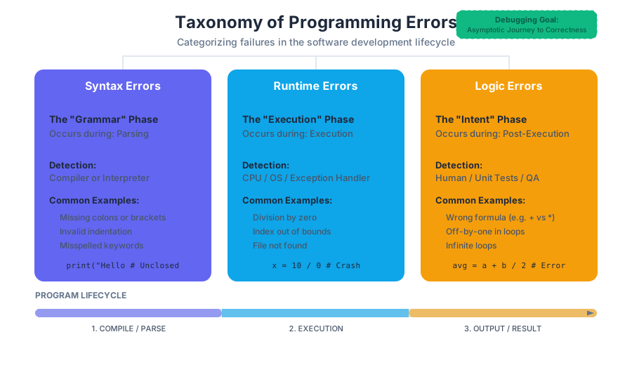
In the realm of computer science, the transition from a conceptual algorithm to a functional program is rarely a linear path. It is an asymptotic journey toward correctness, mediated by a process known as debugging. Debugging is not merely the act of "fixing mistakes"; it is a rigorous, scientific application of the deductive method to identify, isolate, and rectify flaws within a system's state or logic.
The term "bug" was famously popularized by Admiral Grace Hopper in 1947 when a literal moth caused a failure in the Harvard Mark II computer. However, in modern software engineering, a bug represents a discrepancy between the expected behavior defined by the requirements and the actual behavior exhibited by the executed code. To master debugging, one must first categorize the failures encountered into three fundamental taxonomies: Syntax Errors, Runtime Errors, and Logic Errors.
Why Debugging Matters
The cost of software defects increases exponentially as a project moves through the lifecycle. An error caught during the initial coding phase (Iterative Development) costs significantly less to fix than an error discovered in production. Beyond economics, debugging fosters a deep mental model of how the computer interprets instructions. As a professor would argue, you do not truly understand a programming language until you understand how it breaks.
### Syntax Errors: The Grammar of Code
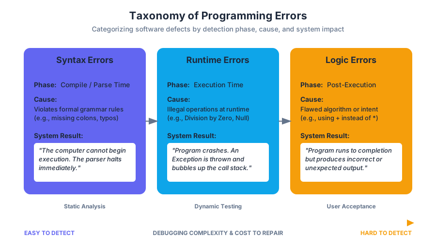
A Syntax Error occurs when the source code violates the formal rules of the programming language's grammar. Every programming language is a "formal language," meaning it has a strictly defined set of symbols and rules for how those symbols can be combined.
The Mechanics of Syntax Analysis
When you attempt to run a program, the Interpreter (in Python) or Compiler (in C/Java) performs a process called Lexical Analysis and Parsing.
- Lexical Analysis: The engine breaks the code into "tokens" (keywords, variables, operators).
- Parsing: The engine checks if these tokens follow the language's Context-Free Grammar. If the parser encounters a token it does not expect, it throws a
SyntaxErrorand halts execution immediately.
Definition: A Syntax Error is a compile-time (or parse-time) error that prevents the program from ever beginning execution. The computer cannot "guess" what you meant; it requires absolute structural precision.
Common Syntax Error Categories
| Error Type | Description | Example (Python) |
|---|---|---|
| Missing Delimiters | Forgetting parentheses, brackets, or quotes. | print("Hello |
| Invalid Indentation | Inconsistent spacing in block-based languages. | if True:\nprint(1) |
| Keyword Misuse | Using reserved words incorrectly. | class = 5 |
| Operator Misplacement | Using operators in a way that violates math/logic. | x = 5 + * 2 |
Code Example 1: Low-Level Syntax and Structure (Python)
The following code demonstrates a script that would fail the parsing phase due to multiple structural violations.
# This script contains intentional Syntax Errors for pedagogical analysis
def calculate_area(radius)
    # Error 1: Missing colon (:) after function definition
    pi = 3.14159
    return pi * radius ** 2

def main():
    try:
        # Error 2: Missing closing parenthesis in the input call
        r = float(input("Enter radius: "
        print(f"Area: {calculate_area(r)}")
    except ValueError:
        print("Invalid input")

# Error 3: Improper indentation (Logic/Syntax hybrid in Python)
if __name__ == "__main__":
main()
### Runtime Errors: The Unexpected Halt
A Runtime Error (often called an Exception) is an error that occurs while the program is running. Unlike syntax errors, the code is grammatically correct and passes the parsing phase. However, during execution, the program reaches a state that the computer cannot handle.
The Anatomy of an Exception
When a runtime error occurs, the environment generates an Exception Object. This object "bubbles up" through the Call Stack—the history of function calls currently active. If the programmer does not "catch" the exception using a try-catch block, the program terminates and prints a Stack Trace.
Mathematical Derivation of a Runtime Error
Consider the function $f(x, y) = \frac{x}{y}$.
In mathematics, the domain of this function excludes $y=0$. In a computer, if a variable y is assigned the value 0 through user input or calculation, the CPU's Arithmetic Logic Unit (ALU) cannot complete the operation, triggering a ZeroDivisionError.
Common Runtime Errors
| Exception Name | Cause | Prevention Strategy |
|---|---|---|
ZeroDivisionError |
Division by zero. | Check if denominator $\neq 0$ before dividing. |
TypeError |
Operation on incompatible types. | Use isinstance() or type-hinting. |
IndexError |
Accessing a list index that doesn't exist. | Check len(list) before access. |
FileNotFoundError |
Attempting to open a non-existent file. | Use os.path.exists(). |
Code Example 2: Low-Level Memory and Runtime Faults (C)
In lower-level languages like C, runtime errors often manifest as "Segmentation Faults" when the program tries to access memory it doesn't own.
#include <stdio.h>
#include <stdlib.h>

/**
 * Demonstrates a Runtime Error (Segmentation Fault)
 * via null pointer dereference.
 */
int main() {
    int *ptr = NULL; // Initialize a pointer to nothing

    printf("Attempting to access memory at NULL...\n");

    // RUNTIME ERROR: The hardware prevents accessing address 0x0
    // This will cause the OS to send a SIGSEGV signal to the process.
    *ptr = 10;

    printf("This line will never be reached.\n");
    return 0;
}
### Logic Errors: The Silent Killer
A Logic Error is the most insidious type of bug. The program runs without crashing and produces output, but the output is incorrect. The computer is doing exactly what you told it to do, but what you told it to do is not what you intended.
Why Logic Errors Occur
Logic errors usually stem from a misunderstanding of the algorithm or a "slip" in implementation. Common causes include:
- Off-by-one errors: Iterating $n$ times instead of $n-1$.
- Operator Precedence: Forgetting that multiplication happens before addition.
- Boolean Logic Flaws: Using
ANDwhenORwas required.
Worked Example: The Average Calculation
Suppose you want to calculate the average of two numbers, $a$ and $b$. The mathematical formula is: $Avg = \frac{a + b}{2}$.
If a programmer writes:
average = a + b / 2
The computer follows the Order of Operations (PEMDAS/BODMAS):
b / 2is calculated first.ais added to that result. The result is $a + \frac{b}{2}$, which is incorrect.
Code Example 3: Algorithmic Logic Error (Pseudocode/Math)
This example demonstrates a logic error in a binary search algorithm where the midpoint calculation causes an infinite loop or a missed element.
ALGORITHM BinarySearch(list, target):
    low = 0
    high = length(list)  // LOGIC ERROR: Should be length - 1

    WHILE low <= high:
        mid = (low + high) / 2

        IF list[mid] == target:
            RETURN mid
        ELSE IF list[mid] < target:
            low = mid   // LOGIC ERROR: Should be mid + 1 to avoid infinite loop
        ELSE:
            high = mid  // LOGIC ERROR: Should be mid - 1

    RETURN -1
### Iterative Development: The Debugging Workflow
To combat these errors, senior engineers employ Iterative Development. Instead of writing 500 lines of code and then trying to run it (the "Big Bang" approach), you write a small "chunk" (5-10 lines), test it immediately, and then move on.
The Red-Green-Refactor Cycle
- Red: Write a test or a small piece of code that you expect to fail or be incomplete.
- Green: Write just enough code to make it work correctly.
- Refactor: Clean up the code, improve variable names, and add comments while ensuring it still works.
Debugging Strategies Comparison
| Strategy | Description | Best For |
|---|---|---|
| Rubber Ducking | Explaining your code line-by-line to an inanimate object. | Logic Errors |
| Print Debugging | Inserting print() statements to track variable states. |
Runtime Errors |
| Unit Testing | Writing small scripts to test individual functions. | Regression Prevention |
| IDE Debuggers | Using tools to pause execution and inspect memory. | Complex State Issues |
### Comments: Documenting the "Why"
Comments are lines of text in the source code that are ignored by the compiler or interpreter. They are written for humans, not machines.
The Purpose of Comments
- Explain Intent: Don't explain what the code does (the code does that); explain why you chose a specific approach.
- Temporary Disabling: During debugging, you can "comment out" a line of code to see if the error persists without it.
- Metadata: Providing author info, dates, and license details.
Theorem of Self-Documenting Code: While comments are vital, the best code is "self-documenting"—meaning variable names like
user_ageare so clear that a comment explaining them is redundant.
Code Example 4: Professional Scripting and Commenting (Bash)
This DevOps script uses comments to explain complex shell interactions and provide usage instructions.
#!/bin/bash

# =================================================================
# SCRIPT: backup_db.sh
# DESCRIPTION: Performs a compressed backup of the production DB.
# AUTHOR: Senior Engineer
# =================================================================

# Define the target directory; ensure it exists
BACKUP_DIR="/var/backups/db"

# Check if the user has root privileges (Runtime check)
if [[ $EUID -ne 0 ]]; then
   echo "This script must be run as root"
   exit 1 # Exit with error code
fi

# Iterate through databases and compress
# NOTE: We exclude the 'temp' database as per Jira ticket #402
for db in $(ls /data/db_files); do
    if [ "$db" != "temp" ]; then
        echo "Backing up: $db"
        tar -czf "$BACKUP_DIR/$db.tar.gz" "/data/db_files/$db"
    fi
done

# TODO: Add logic to sync with AWS S3 bucket in Unit 2
### Common Pitfalls and Misconceptions
- The "It works on my machine" fallacy: Just because a program runs without runtime errors doesn't mean it is correct. Logic errors can hide in specific data sets.
- Over-commenting: Writing
# increment x by 1abovex += 1adds "noise" to the file. Only comment on non-obvious logic. - Confusing Syntax and Logic: Beginners often think a
SyntaxErroris a sign of being a "bad programmer." In reality, syntax errors are trivial. Logic errors are where the real engineering challenge lies. - Ignoring the Stack Trace: When a runtime error occurs, the computer gives you the exact line number and the reason. Beginners often close the error window in frustration; experts read the last three lines of the trace carefully.
### Summary of Error Characteristics
| Feature | Syntax Error | Runtime Error | Logic Error |
|---|---|---|---|
| When it's found | Before the program starts. | While the program is running. | After the program finishes. |
| Who finds it | The Compiler / Interpreter. | The Computer / CPU. | The User / Programmer. |
| Severity | High (Prevents execution). | High (Crashes program). | Variable (Can be catastrophic). |
| Ease of Fix | Easy (Follow the line number). | Moderate (Follow the trace). | Hard (Requires deep analysis). |
Unit 2: Conditional Logic and Branching
Key concepts: Boolean expressions · Comparison operators · if-elif-else statements · Logical operators (and, or, not) · Nested conditionals
Explores how computers make decisions using selection and branching logic.
Unit 2: Conditional Logic and Branching
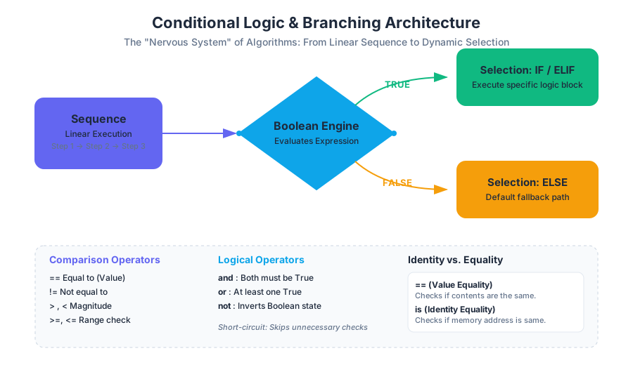
In the foundational study of computation, we transition from Sequence—the linear execution of instructions—to Selection. Conditional logic is the mechanism by which a program evaluates the state of its environment and chooses a specific path of execution. This "branching" capability transforms a static script into a dynamic, "intelligent" system capable of responding to varying inputs and edge cases.
As a professor of computer science, I often describe conditional logic as the "nervous system" of an algorithm. Without it, software is merely a calculator; with it, software becomes a decision-engine. This unit explores the mathematical underpinnings of Boolean algebra, the syntax of branching structures, and the ethical implications of the logic we encode.
### Boolean Expressions and Comparison Operators
At the heart of every decision lies a Boolean Expression: a statement that evaluates to exactly one of two states: True or False. Named after the mathematician George Boole, these expressions form the basis of all modern digital logic.
The Mechanics of Comparison
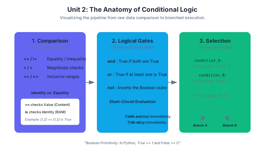
Comparison operators are the tools we use to generate Boolean values by relating two pieces of data. In Python and most C-style languages, these operators allow us to test for equality, inequality, and magnitude.
| Operator | Description | Mathematical Notation | Example (x=10, y=20) |
Result |
|---|---|---|---|---|
== |
Equal to | $x = y$ | x == y |
False |
!= |
Not equal to | $x \neq y$ | x != y |
True |
> |
Greater than | $x > y$ | x > y |
False |
< |
Less than | $x < y$ | x < y |
True |
>= |
Greater than or equal to | $x \geq y$ | x >= 10 |
True |
<= |
Less than or equal to | $x \leq y$ | y <= 15 |
False |
The Identity vs. Equality Distinction
A common pitfall for senior engineers and students alike is the distinction between Value Equality (==) and Identity Equality (is).
==checks if the contents of two objects are the same.ischecks if two variables point to the same memory address (location in RAM).
Theorem of Boolean Primitivity: In Python, the
booltype is a specialized subclass ofint.Trueis numerically equivalent to1, andFalseis equivalent to0. This allows for "Boolean Arithmetic," though it is generally discouraged in clean code for the sake of readability.
# First code block: Low-level implementation of a validation engine
# This demonstrates complex comparison and type-checking logic.

def validate_system_state(temperature, pressure, threshold_map):
    """
    Evaluates hardware safety parameters using comparison operators.
    Returns a status code based on Boolean evaluation.
    """
    # Type checking using identity and built-in functions
    if type(threshold_map) is not dict:
        return "ERR_INVALID_CONFIG"

    # Magnitude comparisons
    is_overheating = temperature > threshold_map.get("max_temp", 100)
    is_pressurized = pressure >= threshold_map.get("min_pressure", 20)

    # Value equality check
    system_ready = (threshold_map.get("status") == "ACTIVE")

    if is_overheating:
        return "CRITICAL_HALT"
    elif not is_pressurized:
        return "LOW_PRESSURE_WARNING"
    elif system_ready:
        return "OPERATIONAL"
    else:
        return "IDLE"

# Example usage
config = {"max_temp": 85, "min_pressure": 30, "status": "ACTIVE"}
print(validate_system_state(90, 35, config)) # Output: CRITICAL_HALT
### Logical Operators (and, or, not)
While comparison operators compare values, Logical Operators combine multiple Boolean expressions into a single, complex condition. This allows for the creation of sophisticated business rules and multi-variable filters.
The Three Pillars of Logic
and(Conjunction): ReturnsTrueonly if both operands areTrue.or(Disjunction): ReturnsTrueif at least one operand isTrue.not(Negation): Inverts the Boolean value (TruebecomesFalse).
Truth Tables
To understand how these operators behave under all possible inputs, we use Truth Tables.
| A | B | A and B | A or B | not A |
|---|---|---|---|---|
True |
True |
True |
True |
False |
True |
False |
False |
True |
False |
False |
True |
False |
True |
True |
False |
False |
False |
False |
True |
Short-Circuit Evaluation
Modern interpreters use a performance optimization called Short-Circuit Evaluation.
- In an
andexpression, if the first operand isFalse, the entire expression is immediatelyFalse, and the second operand is never evaluated. - In an
orexpression, if the first operand isTrue, the entire expression is immediatelyTrue.
This is critical for preventing errors. For example: if (count != 0) and (total / count > 5): will not crash with a "Division by Zero" error because the second half is skipped if count is 0.
\text{De Morgan's Laws for Logic Simplification:} \\
\neg(A \land B) \iff (\neg A) \lor (\neg B) \\
\neg(A \lor B) \iff (\neg A) \land (\neg B)
# Second code block: Mathematical derivation and Pseudocode
# Demonstrating the logic of a multi-factor authentication (MFA) check

ALGORITHM CheckAccess(user, session, device)
    // Propositional Logic Representation:
    // Access = (IsAuthenticated AND (IsTrustedDevice OR HasMFA)) AND NOT IsAccountLocked

    LET auth = user.is_authenticated
    LET trusted = device.is_recognized
    LET mfa = session.mfa_completed
    LET locked = user.is_locked

    IF (auth AND (trusted OR mfa)) AND NOT locked THEN
        RETURN AccessGranted
    ELSE
        RETURN AccessDenied
    END IF
END ALGORITHM
### The if-elif-else Structure
The if statement is the primary control structure for branching. It allows the program to skip blocks of code entirely if a condition is not met.
Syntax and Semantic Whitespace
In Python, the structure is defined by indentation. Unlike C++ or Java, which use curly braces {} to define blocks, Python uses whitespace. This enforces readability but requires strict attention to formatting.
if: The entry point. If the condition isTrue, the block executes.elif(else if): Checked only if the precedingifandelifstatements wereFalse. You can have an arbitrary number of these.else: The "catch-all" block. It executes only if every condition above it failed.
Mutual Exclusivity
In an if-elif-else chain, the blocks are mutually exclusive. Only the first condition that evaluates to True will run. Even if subsequent elif conditions are also True, they will be ignored.
| Structure | Use Case | Execution Flow |
|---|---|---|
Simple if |
Optional action | Runs 0 or 1 block |
if-else |
Binary choice | Runs exactly 1 block |
if-elif-else |
Multiple categories | Runs exactly 1 block |
Multiple ifs |
Independent checks | Runs 0 to N blocks |
# Third code block: Real-world usage (Shell Scripting)
# Checking system environment variables and file permissions

#!/bin/bash

FILE_PATH="/etc/config_data.json"

if [ ! -f "$FILE_PATH" ]; then
    echo "Error: Configuration file missing at $FILE_PATH"
    exit 1
elif [ ! -r "$FILE_PATH" ]; then
    echo "Error: File exists but is not readable. Check permissions."
    exit 1
else
    echo "Success: System ready to load configuration."
    # Logic to parse JSON would go here
fi
### Nested Conditionals and Logic Flattening
Nested Conditionals occur when an if statement is placed inside another if statement. This is used to model hierarchical decisions where a second condition only matters if the first one is true.
The Complexity Problem
While powerful, nesting can lead to the "Arrow Anti-pattern" (or "Pyramid of Doom"), where code drifts further and further to the right of the screen. This makes the logic difficult to follow and debug.
The Zen of Python Rule: "Flat is better than nested."
Refactoring with Guard Clauses
Professional engineers often "flatten" nested logic by using Guard Clauses. A guard clause handles the edge case or error condition at the beginning of a function and exits early, keeping the "happy path" (the main logic) at the lowest level of indentation.
/* Fourth code block: Performance variant in C
   Comparing nested logic vs. a Switch statement for discrete values */

#include <stdio.h>

void process_status_nested(int code) {
    // Nested approach (Harder to read)
    if (code >= 200) {
        if (code < 300) {
            printf("Success\n");
        } else {
            if (code < 400) {
                printf("Redirect\n");
            } else {
                printf("Error\n");
            }
        }
    }
}

void process_status_switch(int code) {
    // Switch approach (More performant for specific integer branches)
    switch(code) {
        case 200: printf("OK\n"); break;
        case 404: printf("Not Found\n"); break;
        case 500: printf("Server Error\n"); break;
        default:  printf("Unknown Status\n");
    }
}
### Algorithmic Bias in Conditional Logic
As we teach computers to make decisions, we must acknowledge that logic is not always neutral. Algorithmic Bias occurs when the conditions we program (or the data we use to train them) result in unfair treatment of certain groups.
How Bias Enters the Code
- Proxy Variables: Using a variable like "Zip Code" as a condition might inadvertently act as a proxy for race or socioeconomic status.
- Incomplete Logic: An
if-elsestructure that doesn't account for cultural naming conventions (e.g., assuming everyone has exactly two names) can exclude users. - Threshold Setting: Setting a "credit score" threshold for a loan might seem objective, but if the underlying system for calculating that score is biased, the conditional logic propagates that bias.
Mitigation Strategies
- Edge Case Testing: Specifically testing the logic against diverse datasets.
- Transparency: Documenting why specific thresholds (e.g.,
if score > 700) were chosen. - Human-in-the-loop: Using conditionals to flag cases for human review rather than making final, irreversible decisions.
### Common Pitfalls and Troubleshooting
Even experienced developers encounter bugs in conditional branching. Here are the most frequent errors:
- The Assignment vs. Equality Trap:
- Using
if x = 10:(assignment) instead ofif x == 10:(comparison). Many languages (like Python) throw a syntax error here to protect you, but in C, this is a valid (and dangerous) statement.
- Using
- Overlapping Conditions:
if score > 70: ... elif score > 80: ...- In this case, a score of 85 will trigger the first block (
> 70) and never reach the> 80block. Order matters.
- Floating Point Comparisons:
- Comparing floats for exact equality (
0.1 + 0.2 == 0.3) often returnsFalsedue to precision limits. Always use a small tolerance:if abs(a - b) < 0.0001:.
- Comparing floats for exact equality (
- Dangling Else:
- In languages without strict indentation, an
elsemight attach to the wrongif. Python's whitespace rules prevent this, but it requires the developer to be diligent with their tabs/spaces.
- In languages without strict indentation, an
| Pitfall | Example | Correction |
|---|---|---|
| Assignment Error | if x = 5: |
if x == 5: |
| Logic Order | if x > 0: ... elif x > 10: |
if x > 10: ... elif x > 0: |
| Float Equality | if price == 19.99: |
if abs(price - 19.99) < 0.01: |
| Redundant Booleans | if is_valid == True: |
if is_valid: |
Unit 3: Loops and Simulations
Key concepts: While loops · For loops with range · Module imports (random) · Loop control (break and continue) · Population dynamics simulations
Focuses on automating repetitive tasks and simulating complex phenomena using loops.
Unit 3: Loops and Simulations
Iteration is the engine of computation. While the previous units focused on state (variables) and selection (conditionals), Unit 3 introduces the ability to repeat logic dynamically. In computer science, we transition from writing linear scripts to designing algorithms—procedures that can handle arbitrary scales of data and time.
This unit explores the two primary forms of iteration: indefinite iteration (where the number of repetitions is unknown at the start) and definite iteration (where we iterate over a known sequence). We will then synthesize these concepts with stochasticity (randomness) to build simulations of complex systems, such as population dynamics and Monte Carlo models.
3.1 Indefinite Iteration: The While Loop
The while loop is the most fundamental looping construct. It functions as a "repeated if statement." As long as a specified Boolean condition evaluates to True, the code block within the loop executes. Once the condition becomes False, the program pointer moves to the next instruction outside the loop.
3.1.1 Mechanics and Syntax
A while loop consists of a loop header and a loop body. The header contains the condition, and the body contains the instructions.
The Halting Problem: In theoretical computer science, determining whether a given program will eventually stop (halt) or run forever is undecidable. When writing
whileloops, the burden is on the programmer to ensure the loop condition eventually evaluates toFalse.
| Component | Role | Risk if Mismanaged |
|---|---|---|
| Initialization | Setting the starting state of the control variable. | Uninitialized variable error. |
| Condition | The Boolean expression checked before every iteration. | Logic error leading to zero iterations. |
| Update | Modifying the state so the condition eventually fails. | Infinite Loop: The program hangs indefinitely. |
3.1.2 Implementation: The Sentinel Pattern
A common use for while loops is processing user input or data streams where the end-point is marked by a specific value, known as a sentinel.
# Implementation of a robust data accumulator with a sentinel value
def collect_sensor_data():
    data_points = []
    sentinel = -999.0  # Value indicating end of stream

    print(f"Enter sensor readings (type {sentinel} to stop):")

    while True:
        try:
            raw_input = input("> ")
            val = float(raw_input)

            if val == sentinel:
                break  # Exit loop immediately

            data_points.append(val)

        except ValueError:
            print("Invalid input. Please enter a numeric value.")

    return data_points

# Calculate average from the collected data
readings = collect_sensor_data()
if readings:
    print(f"Mean Reading: {sum(readings) / len(readings):.2f}")
3.2 Definite Iteration: For Loops and the Range Object
While while loops are powerful for state-based repetition, for loops are the standard for iterating over a sequence of values. In Python, the for loop is an iterator-based construct, meaning it pulls items from a collection one by one.
3.2.1 The range() Function
The range() function is a built-in generator that produces a sequence of integers. It is highly memory-efficient because it does not store the entire list of numbers in memory; instead, it calculates the next number on demand.
The range(start, stop, step) function follows these mathematical rules:
- Start: Inclusive.
- Stop: Exclusive (the loop stops before reaching this value).
- Step: The increment between values (can be negative for counting down).
Algorithm: Range Sequence Generation
Input: start (a), stop (b), step (s)
Output: A sequence S where S_i = a + i*s
Constraint:
    If s > 0: a + i*s < b
    If s < s: a + i*s > b
3.2.2 Comparison of Range Parameters
| Syntax | Sequence Produced | Use Case |
|---|---|---|
range(5) |
0, 1, 2, 3, 4 | Simple repetition $N$ times. |
range(1, 6) |
1, 2, 3, 4, 5 | Iterating through 1-based indices. |
range(0, 10, 2) |
0, 2, 4, 6, 8 | Iterating through even numbers. |
range(10, 0, -1) |
10, 9, 8, ..., 1 | Counting down (e.g., a timer). |
3.3 Loop Control: Break and Continue
Sometimes, the standard entry/exit logic of a loop is insufficient. We use control flow statements to alter the loop's execution path mid-stream.
break: Immediately terminates the innermost loop. Execution resumes at the first statement after the loop block.continue: Skips the remainder of the current loop body and jumps back to the header for the next iteration (re-evaluating the condition).
3.2.3 Low-Level Logic Comparison
To understand how these work at the hardware level, we can look at how a high-level for loop with a break might be represented in a lower-level language like C, which maps more closely to assembly jumps.
#include <stdio.h>

// Demonstrating loop control at a low level
int main() {
    int target = 7;

    // For loop: (initialization; condition; increment)
    for (int i = 0; i < 10; i++) {
        if (i % 2 == 0) {
            // 'continue' equivalent: jump to increment
            continue;
        }

        if (i == target) {
            // 'break' equivalent: jump out of loop
            break;
        }

        printf("Processing odd number: %d\n", i);
    }

    return 0;
}
3.4 Stochasticity and the random Module
Simulations require unpredictability. Since computers are deterministic machines, they use Pseudorandom Number Generators (PRNGs). These are mathematical algorithms that produce a sequence of numbers that appear random but are actually determined by an initial value called a seed.
3.4.1 Key Functions in random
| Function | Output Type | Description |
|---|---|---|
random.random() |
Float | Returns a value in the range $[0.0, 1.0)$. |
random.randint(a, b) |
Integer | Returns a value in the range $[a, b]$ (inclusive). |
random.uniform(a, b) |
Float | Returns a value in the range $[a, b]$. |
random.choice(seq) |
Element | Returns a random element from a non-empty sequence. |
Pro-Tip: For scientific simulations, always set a seed using
random.seed(value). This ensures your results are reproducible, allowing other researchers to generate the exact same "random" sequence.
3.5 Population Dynamics and Simulations
A simulation is a computational model of a real-world process. In biology and sociology, we often simulate population dynamics to predict how a group of organisms changes over time based on birth rates, death rates, and environmental carrying capacity.
3.5.1 The Discrete-Time Model
In a loop-based simulation, we treat time as a series of discrete "steps" (e.g., years or generations). At each step, we apply a set of rules to update the state.
The Malthusian Growth Formula: $$P_{t+1} = P_t + (r \times P_t)$$ Where:
- $P_t$ is the population at time $t$.
- $r$ is the growth rate (birth rate - death rate).
3.5.2 Complex Simulation: Logistic Growth with Stochasticity
In reality, populations don't grow forever. They are limited by a Carrying Capacity (K). Furthermore, random events (famine, disease) introduce variance.
import random

def simulate_population(initial_pop, growth_rate, carrying_capacity, years):
    """
    Simulates population growth using the Logistic Model with
    stochastic environmental shocks.
    """
    population = initial_pop
    history = [initial_pop]

    print(f"{'Year':<5} | {'Population':<12} | {'Event'}")
    print("-" * 35)

    for year in range(1, years + 1):
        # 1. Calculate deterministic growth (Logistic Equation)
        # Growth slows as population approaches K
        growth = growth_rate * population * (1 - population / carrying_capacity)

        # 2. Introduce Stochasticity (Random Environmental Shock)
        # 10% chance of a "bad year" where 20% of the population is lost
        event = "Stable"
        if random.random() < 0.10:
            growth -= (population * 0.20)
            event = "Famine!"

        population += int(growth)

        # Ensure population doesn't drop below zero
        population = max(0, population)
        history.append(population)

        print(f"{year:<5} | {population:<12} | {event}")

        if population == 0:
            print("Extinction event occurred.")
            break

    return history

# Execution
results = simulate_population(initial_pop=50, growth_rate=0.5, carrying_capacity=1000, years=50)
3.6 Complexity and Nested Loops
When a loop is placed inside another loop, it is called a nested loop. These are essential for working with multi-dimensional data (like grids or matrices) but can lead to performance bottlenecks.
3.6.1 Big O Notation and Performance
The efficiency of a loop is often measured in Big O notation, which describes how the execution time grows as the input size ($n$) increases.
| Structure | Complexity | Description |
|---|---|---|
| Single Loop | $O(n)$ | Linear time. If $n$ doubles, time doubles. |
| Nested Loop (2 levels) | $O(n^2)$ | Quadratic time. If $n$ doubles, time quadruples. |
| Nested Loop (3 levels) | $O(n^3)$ | Cubic time. Common in 3D simulations. |
3.6.2 Example: Coordinate Grid Generation
To simulate a 2D environment (like a forest or a game map), we use nested loops to iterate over $x$ and $y$ coordinates.
# Example of how a shell script might invoke a Python simulation
# with different parameters to conduct a sensitivity analysis.

for rate in 0.1 0.2 0.3 0.4 0.5; do
    echo "Running simulation with growth rate: $rate"
    python3 population_sim.py --rate $rate --output "results_$rate.csv"
done

echo "All simulations complete. Analyzing data..."
3.7 Common Pitfalls in Loop Design
- Off-by-One Errors: Using
range(10)when you need the number 10 included. Remember thatstopis exclusive. - Modifying the Iterator: Never add or remove items from a list while you are iterating over it with a
forloop. This leads to skipped elements or runtime errors. - Floating Point Precision in Conditions: Avoid using
while x != 1.0:because floating-point math is imprecise (e.g.,0.1 + 0.2is actually0.30000000000000004). Use inequalities likewhile x < 1.0:. - Infinite While Loops: Forgetting to update the control variable inside the loop body.
Summary of Unit 3
Loops transform code from a static list of instructions into a dynamic system capable of processing vast amounts of information. By combining while and for loops with the random module, we can move beyond simple arithmetic and begin modeling the complexity of the natural world.
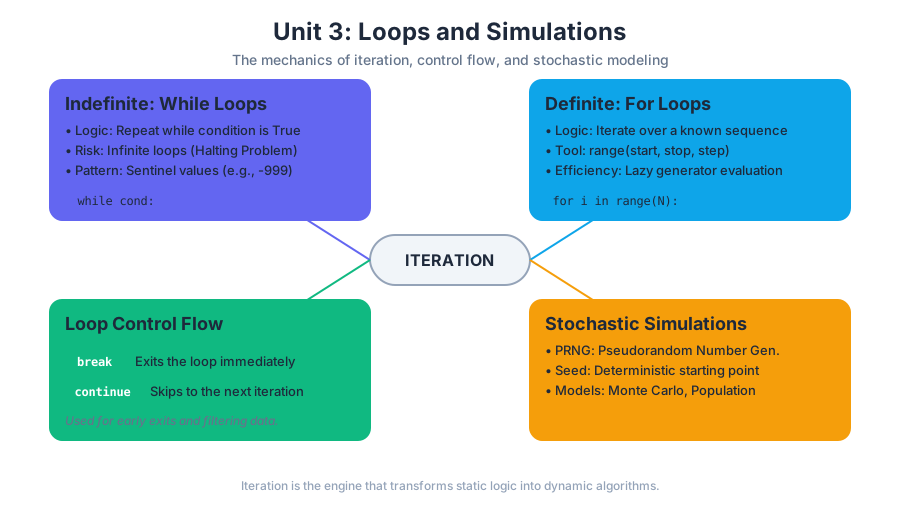
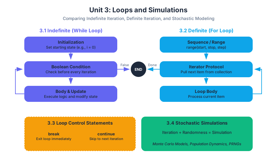
Unit 4: Functions and Modularity
Key concepts: Function definitions and parameters · Local and global scope · Return values · Unit testing · Code organization
Teaches how to break down complex code into smaller, reusable, and organized modules.
Unit 4: Functions and Modularity
The Architecture of Abstraction: An Introduction to Modularity
In the early stages of programming, code is often written as a linear script—a single, sequential list of instructions executed from top to bottom. While sufficient for trivial tasks, this "spaghetti" approach fails as complexity scales. Modularity is the engineering principle of breaking a complex system into smaller, self-contained, and interchangeable parts. In computer science, the primary unit of modularity is the function.
A function is a named, reusable block of code that performs a specific action. By encapsulating logic within functions, we achieve abstraction: the ability to use a complex tool without needing to understand its internal mechanics at every moment. This is analogous to a pilot using a cockpit instrument; they need to know the input (altitude) and the output (reading), but not the specific circuitry inside the gauge.
1. Function Definitions and Parameters
At its core, a function is a mapping between an input space and an output space. In Python, we define this mapping using the def keyword, followed by a unique identifier and a set of formal parameters.
1.1 The Anatomy of a Function
A robust function definition consists of the header, the docstring (documentation), the body, and the return statement. The parameters act as placeholders for the data the function requires to operate.
Definition: Formal Parameter vs. Actual Argument A formal parameter is the variable defined in the function signature (the "hole" in the machine). An actual argument is the real value passed into that "hole" during a function call.
1.2 Mechanics of Parameter Passing
Python utilizes a mechanism often called pass-by-object-reference. When you pass an argument to a function, you are passing a reference to the object, not a copy of the object itself. However, whether the original data can be changed depends on whether the object is mutable (like a list) or immutable (like an integer or string).
| Component | Syntax Example | Purpose |
|---|---|---|
| Keyword | def |
Signals the start of a function definition. |
| Identifier | calculate_entropy |
The name used to invoke the function later. |
| Parameters | (data, base=2) |
Variables that receive input values. |
| Docstring | """Computes...""" |
Human-readable explanation of the function's behavior. |
| Body | return -sum(p...) |
The algorithmic logic of the function. |
| Return | return result |
The mechanism for sending data back to the caller. |
1.3 Implementation: Non-Trivial Algorithm
The following example demonstrates a function implementing Simpson's Rule for numerical integration. This is a non-trivial mathematical algorithm that requires modularity to remain readable.
import math

def simpsons_rule(f, a, b, n):
    """
    Approximates the definite integral of f from a to b using Simpson's Rule.

    Parameters:
    f (function): The integrand function to be integrated.
    a (float): Lower bound of integration.
    b (float): Upper bound of integration.
    n (int): Number of sub-intervals (must be even).

    Returns:
    float: The approximated area under the curve.
    """
    if n % 2 != 0:
        raise ValueError("n must be an even integer.")

    h = (b - a) / n
    # Initial sum with the endpoints
    integral_sum = f(a) + f(b)

    for i in range(1, n):
        x_i = a + i * h
        if i % 2 == 0:
            # Even indices are multiplied by 2
            integral_sum += 2 * f(x_i)
        else:
            # Odd indices are multiplied by 4
            integral_sum += 4 * f(x_i)

    return (h / 3) * integral_sum

# Usage: Integrate sin(x) from 0 to Pi
result = simpsons_rule(math.sin, 0, math.pi, 100)
print(f"Approximated Integral: {result}")
2. Return Values and Control Flow
A function without a return value is often called a procedure. While procedures are useful for side effects (like printing to a console or saving a file), pure functions rely on return to pass results back to the calling environment.
2.1 The Return Statement as a Jump
When a return statement is executed, two things happen:
- The expression following
returnis evaluated. - The function's execution terminates immediately, and control is handed back to the point where the function was called.
2.2 Multiple Return Values
While many languages restrict functions to a single return value, Python allows returning multiple values by packing them into a tuple. This is mathematically equivalent to returning a single vector in $\mathbb{R}^n$.
2.3 Mathematical Representation
To understand functions at a theoretical level, we can view them through the lens of Lambda Calculus or set theory.
\text{Let } f: X \to Y \text{ be a function where } X \text{ is the domain and } Y \text{ is the codomain.} \\
\text{In programming, we define } f(x) = y \text{ such that:} \\
\forall x \in \text{Inputs}, \exists! y \in \text{Outputs} \\
\text{The 'return' operation is the mapping } x \mapsto y.
| Return Scenario | Behavior | Example |
|---|---|---|
| Explicit Return | Returns the specified value and exits. | return x + y |
| Implicit Return | Returns None after the last line is executed. |
(No return statement) |
| Early Return | Exits the function based on a conditional check. | if error: return None |
| Multiple Return | Returns a tuple of values. | return lat, lon |
3. Scope: Local vs. Global
Scope refers to the region of a program where a specific variable name is valid and accessible. Understanding scope is critical for preventing "name collisions" and managing memory efficiently.
3.1 The LEGB Rule
Python resolves variable names using the LEGB hierarchy. When you reference a variable, Python looks for it in this specific order:
- Local: Variables defined inside the current function.
- Enclosing: Variables in the local scope of any enclosing functions (relevant in nested functions).
- Global: Variables defined at the top level of the script or module.
- Built-in: Names pre-defined by Python (e.g.,
len,range).
3.2 The Lifetime of a Variable
A variable's lifetime is the duration for which it exists in memory. Local variables are created when the function is called and destroyed when the function returns. This is managed via the Call Stack. Each function call creates a new Stack Frame containing its local variables.
3.3 Scope in Action: A Comparison
To illustrate how scope behaves differently across environments, consider how a shell script manages variables compared to a structured programming language.
#!/bin/bash

# Global variable
APP_STATUS="Running"

check_status() {
    # Local variable (using the 'local' keyword)
    local APP_STATUS="Internal Check"
    echo "Inside function: $APP_STATUS"
}

echo "Before function: $APP_STATUS"
check_status
echo "After function: $APP_STATUS"

# Output:
# Before function: Running
# Inside function: Internal Check
# After function: Running
3.4 Common Pitfall: The Global Keyword
While you can modify a global variable from inside a function using the global keyword, it is generally considered bad practice. It creates hidden dependencies that make the code difficult to test and reason about. A function should ideally be a "black box" that only interacts with the outside world through its parameters and return values.
4. Unit Testing and Debugging
As modularity increases, so does the need for verification. Unit Testing is the practice of testing the smallest "units" of code—functions—in isolation.
4.1 The Philosophy of Testing
The goal of a unit test is to prove that for a specific set of inputs, the function produces the expected output. This provides a "safety net" when refactoring code.
4.2 Test Categories
When designing tests, engineers focus on three types of cases:
- Happy Path: Standard, valid inputs.
- Edge Cases: Inputs at the boundaries of validity (e.g., 0, empty strings, very large numbers).
- Corner Cases: Multiple edge cases occurring simultaneously.
| Test Type | Objective | Example for divide(a, b) |
|---|---|---|
| Positive Test | Verify correct functionality. | divide(10, 2) == 5 |
| Negative Test | Verify error handling. | divide(10, 0) raises ZeroDivisionError |
| Boundary Test | Check limits of data types. | divide(2**31, 1) |
4.3 Implementation: Unit Testing with unittest
The following code demonstrates how to structure formal tests for a function that calculates the Fibonacci sequence.
import unittest

def fibonacci(n):
    """Returns the nth Fibonacci number."""
    if not isinstance(n, int) or n < 0:
        raise ValueError("Input must be a non-negative integer.")
    if n == 0: return 0
    if n == 1: return 1

    a, b = 0, 1
    for _ in range(2, n + 1):
        a, b = b, a + b
    return b

class TestFibonacci(unittest.TestCase):
    def test_standard_values(self):
        self.assertEqual(fibonacci(5), 5)
        self.assertEqual(fibonacci(10), 55)

    def test_base_cases(self):
        self.assertEqual(fibonacci(0), 0)
        self.assertEqual(fibonacci(1), 1)

    def test_negative_input(self):
        with self.assertRaises(ValueError):
            fibonacci(-1)

    def test_type_safety(self):
        with self.assertRaises(ValueError):
            fibonacci("five")

if __name__ == '__main__':
    unittest.main()
5. Modularity and Code Organization
Beyond individual functions, modularity extends to how we organize files and libraries. This is the "Macro" view of Unit 4.
5.1 The DRY Principle
DRY stands for Don't Repeat Yourself. If you find yourself copying and pasting the same five lines of code in three different places, those lines should be encapsulated into a function. This ensures that if the logic needs to change, you only have to change it in one place.
5.2 Separation of Concerns (SoC)
A well-organized program separates different types of logic into different modules:
- Data Layer: Functions for reading/writing data.
- Logic Layer: Functions for processing and calculating.
- Presentation Layer: Functions for displaying results to the user.
5.3 Namespace Management
When importing functions from other modules, Python uses namespaces to prevent name collisions. Using import math creates a math namespace, requiring math.sqrt(). This is safer than from math import *, which dumps all names into the global scope and can lead to "shadowing" (where a library function overwrites your own function).
| Strategy | Syntax | Pros | Cons |
|---|---|---|---|
| Module Import | import math |
Clear origin of functions. | Slightly more typing. |
| Specific Import | from math import pi |
Clean code for specific constants. | Risk of name collision. |
| Aliased Import | import pandas as pd |
Shorthand for frequent use. | Can be confusing for beginners. |
Summary of Best Practices
- Keep functions small: A function should do one thing and do it well (The Single Responsibility Principle).
- Use descriptive names:
calculate_tax_rate()is better thancalc(). - Avoid side effects: A function should ideally not modify global variables or external state unless that is its explicit purpose.
- Document everything: Use docstrings to explain the "what" and "why," even if the "how" seems obvious.
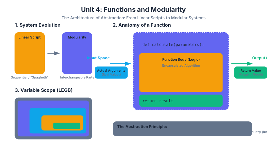
Unit 5: Data Structures - Lists and Sequences
Key concepts: List indexing · Iteration patterns · String immutability · List mutation (append, insert) · The accumulator pattern
Explores how to store and process multiple values using lists and strings.
Unit 5: Data Structures - Lists and Sequences
In the preceding units, we focused on atomic data types—integers, floats, and booleans—which represent single values in isolation. However, computational power is truly realized when we transition from individual data points to sequences. A sequence is an ordered collection of items, allowing us to represent complex structures like a list of temperatures, the characters in a DNA strand, or the pixels in an image.
This unit explores the mechanics of Lists and Strings, the two primary sequence types in Python. We will examine how they are stored in memory, how we can traverse them efficiently, and the fundamental distinction between mutable and immutable data.
1. List Indexing and Memory Architecture
At its core, a list is a contiguous block of memory references. To understand why we access lists the way we do, we must understand the relationship between the index and the physical memory address.
The Zero-Based Indexing Logic
In Python, lists use zero-based indexing. While this can be counterintuitive for beginners, it is rooted in the mathematical definition of an "offset." If a list starts at memory address $B$ (the base address), and each element occupies $S$ bytes, the address of the $i$-th element is calculated as:
$$\text{Address}(i) = B + (i \times S)$$
By starting at index 0, the first element is located exactly at the base address ($B + 0$).
Positive and Negative Indexing
Python provides a dual-indexing system. Positive indices (0 to $n-1$) track the sequence from the beginning, while negative indices (-1 to $-n$) track it from the end.
| Index (Pos) | Index (Neg) | Element Example | Description |
|---|---|---|---|
0 |
-5 |
'P' |
The "Head" of the sequence |
1 |
-4 |
'y' |
Second element |
2 |
-3 |
't' |
Middle element |
3 |
-2 |
'h' |
Second to last |
4 |
-1 |
'o' |
The "Tail" of the sequence |
Slicing: Extracting Sub-sequences
Slicing allows us to extract a portion of a list using the syntax list[start:stop:step].
- Start: The inclusive beginning index.
- Stop: The exclusive ending index (the slice goes up to, but does not include, this index).
- Step: The interval between elements (default is 1).
Theorem of Slicing: The length of a slice
a[i:j]is always $j - i$, provided both indices are within the bounds of the list. This "half-open interval" design simplifies many algorithmic calculations.
# Implementation: Advanced List Slicing and Manipulation
def rotate_list(data, k):
    """
    Rotates a list to the right by k steps.
    Demonstrates slicing and sequence concatenation.
    """
    if not data:
        return data

    n = len(data)
    k = k % n  # Handle cases where k > n

    # The tail becomes the new head
    # The old head follows the tail
    rotated = data[-k:] + data[:-k]
    return rotated

# Example usage
primes = [2, 3, 5, 7, 11, 13]
print(f"Original: {primes}")
print(f"Rotated by 2: {rotate_list(primes, 2)}")
# Output: [11, 13, 2, 3, 5, 7]
2. Iteration Patterns: Traversing Sequences
Iteration is the process of visiting every element in a sequence exactly once. In Python, we distinguish between element-based iteration and index-based iteration.
Element-based (The for-in loop)
This is the most "Pythonic" way to iterate. It abstracts away the index and provides direct access to the object. Use this when you only care about the values, not their positions.
Index-based (The range(len()) pattern)
Sometimes we need the index to modify the list in place or to compare elements at different positions (e.g., checking if list[i] > list[i-1]).
The enumerate Pattern
To get the best of both worlds, enumerate() provides a counter alongside the element.
| Pattern | Syntax | Best Use Case |
|---|---|---|
| Direct | for item in list: |
Reading values, printing, summing. |
| Indexed | for i in range(len(list)): |
Modifying elements, comparing neighbors. |
| Enumerated | for i, item in enumerate(list): |
When both value and position are needed. |
ALGORITHM: Find Max Element
INPUT: A sequence S of n numbers
OUTPUT: The largest number in S

1.  Set max_val = S[0] (Assume first is largest)
2.  FOR each index i from 1 to n-1:
3.      IF S[i] > max_val THEN:
4.          max_val = S[i]
5.  RETURN max_val

COMPLEXITY: O(n) - We must touch every element once.
3. String Immutability vs. List Mutation
One of the most critical distinctions in computer science is between mutable and immutable objects.
Definition: Immutability: An object is immutable if its state cannot be modified after it is created. In Python,
str,int,float, andtupleare immutable.
The String Constraint
If you have a string s = "Python", you cannot perform s[0] = "J". To "change" a string, you must create an entirely new string in memory and reassign the variable name to it. This has significant performance implications for large-scale text processing.
The List Advantage
Lists are mutable. You can change, add, or remove elements without creating a new list object. This makes lists ideal for dynamic data that changes over time.
| Feature | Strings (str) |
Lists (list) |
|---|---|---|
| Mutability | Immutable | Mutable |
| Homogeneity | Usually characters | Can be heterogeneous (mixed types) |
| Memory | Compact, fixed-size | Over-allocated for growth |
| In-place change | Impossible | Possible via append, pop, etc. |
4. List Mutation Methods: Append, Insert, and Beyond
Mutation allows a list to grow and shrink dynamically. Behind the scenes, Python lists are implemented as dynamic arrays.
append(item)
Adds an item to the end of the list. This is an $O(1)$ (constant time) operation on average because Python over-allocates memory to accommodate future growth.
insert(index, item)
Adds an item at a specific position. This is an $O(n)$ operation because every element to the right of the insertion point must be shifted one position in memory.
pop(index) and remove(value)
pop(): Removes and returns the item at an index (default is the last item).remove(): Searches for the first occurrence of a specific value and deletes it.
# Real-world usage: Simulating a Task Queue via CLI
# We use a list to store tasks and 'pop(0)' to process them (FIFO)

# Theoretical Bash representation of list-like processing:
echo "task1,task2,task3" | tr ',' '\n' | while read task; do
    echo "Processing: $task"
    # This mimics iterating through a sequence and performing an action
done
Mutation Performance Table
| Method | Complexity | Description |
|---|---|---|
l.append(x) |
$O(1)$ | Add to end (Efficient) |
l.pop() |
$O(1)$ | Remove from end (Efficient) |
l.insert(0, x) |
$O(n)$ | Add to front (Expensive - requires shifting) |
l.pop(0) |
$O(n)$ | Remove from front (Expensive) |
l.sort() |
$O(n \log n)$ | Reordering elements |
5. The Accumulator Pattern
The Accumulator Pattern is a fundamental algorithmic template used to transform a sequence into a single result or a new, filtered sequence.
Structure of the Pattern:
- Initialize an accumulator variable (e.g.,
total = 0ornew_list = []). - Iterate through the source sequence.
- Update the accumulator based on some logic or condition.
- Return the final state of the accumulator.
Types of Accumulation:
- Summing/Counting: Reducing a list to a single number.
- Filtering: Creating a sub-list that meets specific criteria.
- Mapping: Creating a new list where every element has been transformed.
# Real-World Usage: Data Sanitization and Transformation
def clean_sensor_data(raw_readings, threshold):
    """
    Uses the Accumulator Pattern to filter out noise (values below threshold)
    and normalize the remaining data.
    """
    # 1. Initialize Accumulator
    cleaned_data = []

    # 2. Iterate
    for reading in raw_readings:
        # 3. Logic/Update
        if reading >= threshold:
            # Normalize reading to a 0-1 scale (assuming max 100)
            normalized = reading / 100.0
            cleaned_data.append(normalized)

    # 4. Return result
    return cleaned_data

# Data from a hypothetical temperature sensor
raw_data = [12, 85, 7, 92, 105, 3, 76]
processed = clean_sensor_data(raw_data, 10)
print(f"Processed Readings: {processed}")
6. Common Pitfalls and Edge Cases
1. Modifying a List While Iterating
One of the most common "senior" mistakes is removing items from a list while looping through it.
- The Problem: When you remove an item, the indices of all subsequent items shift. The loop index continues to increment, causing it to skip the element immediately following the deleted one.
- The Solution: Iterate over a copy of the list (
for x in my_list[:]) or use a list comprehension to create a new filtered list.
2. Shallow vs. Deep Copies
When you assign list_b = list_a, you are not creating a new list; you are creating a new reference to the same list in memory. Changing list_b will change list_a. To create a true independent copy, use list_b = list_a.copy().
3. Off-by-One Errors
Because of zero-based indexing, the last element is always at len(my_list) - 1. Attempting to access my_list[len(my_list)] will trigger an IndexError.
Summary of Unit 5
Lists and sequences represent the first step toward handling "Big Data." By understanding the memory implications of indexing, the constraints of string immutability, and the power of the accumulator pattern, programmers can write code that is not only functional but also efficient. Whether you are building a simple calculator or a complex encryption algorithm, these structures form the bedrock of your data architecture.
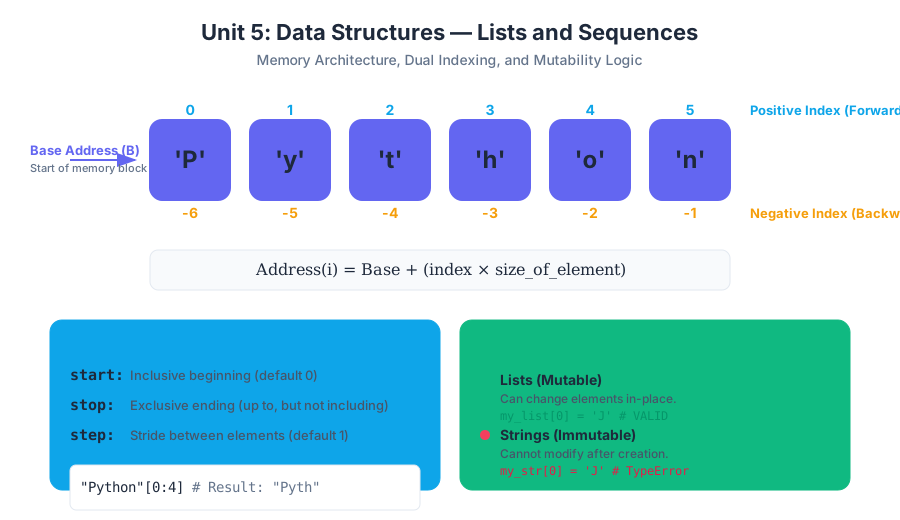
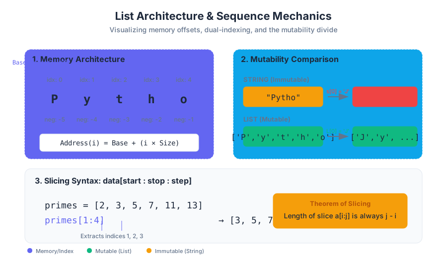
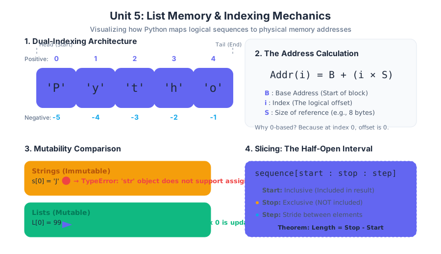
Unit 6: Object-Oriented Programming (OOP)
Key concepts: Classes and Objects · Instance Attributes and State · Methods and Encapsulation · Special Methods (Dunder Methods) · Object Composition
Introduces the OOP paradigm to model real-world entities using classes and objects.
Unit 6: Object-Oriented Programming (OOP)
Object-Oriented Programming (OOP) represents a fundamental shift in the architecture of software. While procedural programming focuses on the sequence of actions (the "how"), OOP focuses on the entities involved (the "what"). By bundling data and the logic that manipulates that data into cohesive units called objects, we create a system that is modular, extensible, and significantly easier to reason about as complexity scales.
1. Classes and Objects: The Blueprint and the Instance
At its core, OOP is a method of abstraction. We define a Class as a programmer-defined blueprint from which individual Objects are created. If a class is the architectural drawing of a house, the object is the physical house built on a specific lot.
What it is
A Class is a logical grouping of data and functions. Mathematically, we can view a class $C$ as a set of potential states $S$ and a set of transitions $M$ (methods) that operate on those states. An Object (or instance) is a concrete realization of that class, occupying a specific block of memory and holding its own unique state.
Why it matters
In large-scale systems, managing global state is a recipe for disaster. OOP solves this by localizing state. Instead of having a variable player_health floating in global scope, it is encapsulated within a Player object. This prevents "spaghetti code" where a change in one part of the program causes unpredictable side effects elsewhere.
How it works: The Instantiation Pipeline
- Definition: The interpreter reads the class definition and stores it in memory.
- Allocation: When
ClassName()is called, the system allocates memory for a new instance. - Initialization: The
__init__method is automatically invoked to set the starting state. - Reference: A reference (memory address) is returned to the variable name.
| Concept | Description | Analogy |
|---|---|---|
| Class | The template/type definition. | The recipe for a cake. |
| Object | The specific instance in memory. | The actual cake on your plate. |
| Instantiation | The process of creating an object. | Baking the cake. |
| Type | The classification of the object. | "Chocolate Cake" vs "Sponge Cake". |
# First code block: Low-level implementation of a complex system
# Modeling a Network Socket Connection with state management

class SecureSocket:
    """A high-level abstraction for a network socket with encryption state."""

    def __init__(self, host: str, port: int):
        self.address = (host, port)
        self.is_connected = False
        self.buffer = []
        self._encryption_key = None  # Internal state

    def connect(self):
        # Logic to establish a handshake
        print(f"Establishing connection to {self.address[0]}...")
        self.is_connected = True
        self._encryption_key = "0xDEADBEEF" # Simulated key exchange

    def send_data(self, payload: str):
        if not self.is_connected:
            raise ConnectionError("Socket must be connected before sending.")
        encrypted = f"[{self._encryption_key}] {payload}"
        self.buffer.append(encrypted)
        print(f"Data buffered: {encrypted}")

# Usage
client = SecureSocket("127.0.0.1", 8080)
client.connect()
client.send_data("Hello, Server!")
2. Instance Attributes and State
The "State" of an object is defined by its Attributes. These are variables that are bound to a specific instance of a class.
The self Keyword
In Python, self is the conventional name for the first parameter of an instance method. It represents the specific instance being acted upon. When you call object.method(), Python automatically passes object as the first argument.
The State Theorem: For any object $O$ of class $C$, the state at time $t$, denoted as $\sigma(O, t)$, is the mapping of all instance attributes to their current values. The behavior of $O$ is a function of both its inputs and its current state $\sigma$.
Class vs. Instance Attributes
It is vital to distinguish between attributes that belong to the class and those that belong to the instance.
| Attribute Type | Scope | Memory Usage | Common Use Case |
|---|---|---|---|
| Instance Attribute | Unique to each object. | Allocated per object. | Names, IDs, health points, coordinates. |
| Class Attribute | Shared by all instances. | Allocated once for the class. | Constants, configuration, instance counters. |
# Second code block: Mathematical/Pseudocode representation of Object State

Definition: Object(S, M)
Let S = {a_1: v_1, a_2: v_2, ... a_n: v_n} be the set of Instance Attributes (State).
Let M = {f_1, f_2, ... f_m} be the set of Methods (Transitions).

Transition Function:
f_i(S, inputs) -> (S', output)

Example: BankAccount
S = {balance: 100}
M = {deposit(amount)}

deposit(S, 50):
    S.balance = S.balance + 50
    Return S' where S'.balance = 150
3. Methods and Encapsulation
Methods define the behavior of an object. Encapsulation is the practice of hiding the internal details of how an object works and exposing only what is necessary through a public interface.
Mechanics of Encapsulation
In many languages (like Java or C++), encapsulation is enforced by keywords like private or protected. Python follows a "consenting adults" philosophy:
- Public:
attribute(Accessible from anywhere). - Protected:
_attribute(A hint that it is internal; should not be accessed outside the class). - Private:
__attribute__(Triggers Name Mangling to prevent accidental overrides in subclasses).
Why Encapsulation Matters
- Integrity: Prevents external code from setting an object into an invalid state (e.g., setting a
BankAccountbalance to a negative number). - Abstraction: The user of the class doesn't need to know how the data is stored, only how to interact with it.
- Maintainability: You can change the internal implementation (e.g., switching from a list to a dictionary) without breaking external code that uses the object.
# Third code block: Real-world usage via CLI and Environment
# Demonstrating how an OOP-based SDK might be configured and used

# 1. Set up environment
export API_KEY="sk-12345"
export DB_URL="postgres://user:pass@localhost:5432/prod"

# 2. Pseudocode for a CLI tool using an OOP Controller
# $ python-cli upload --file data.csv --target s3://my-bucket

# Inside the implementation:
# storage = S3Backend(bucket="my-bucket")
# storage.authenticate(os.getenv("API_KEY"))
# storage.upload("data.csv")
4. Special Methods (Dunder Methods)
Dunder Methods (Double Underscore methods) are the "magic" hooks that allow your custom objects to interact with Python's built-in syntax. They implement what is known as the Python Data Model.
Common Dunder Methods
By implementing these, you make your objects feel like native Python types.
| Method | Purpose | Triggered By |
|---|---|---|
__init__ |
Constructor | obj = ClassName() |
__str__ |
User-friendly string | print(obj) or str(obj) |
__repr__ |
Developer-friendly string | Inspecting in REPL or repr(obj) |
__len__ |
Returns length | len(obj) |
__add__ |
Operator overloading | obj1 + obj2 |
__getitem__ |
Indexing/Slicing | obj[key] |
Worked Example: A Vector Class
Consider a 2D Vector. Without dunder methods, adding two vectors would look like v1.add(v2). With __add__, it becomes v1 + v2, which is much more readable.
# Fourth code block: Dunder methods and Operator Overloading

class Vector2D:
    def __init__(self, x, y):
        self.x = x
        self.y = y

    def __add__(self, other):
        if not isinstance(other, Vector2D):
            return NotImplemented
        return Vector2D(self.x + other.x, self.y + other.y)

    def __repr__(self):
        return f"Vector2D({self.x}, {self.y})"

    def __eq__(self, other):
        return self.x == other.x and self.y == other.y

# Execution
v1 = Vector2D(2, 3)
v2 = Vector2D(4, 5)
v3 = v1 + v2  # Triggers __add__
print(v3)     # Triggers __repr__ -> Vector2D(6, 8)
5. Object Composition
Composition is a design principle where a complex object is built by combining simpler objects. It represents a "has-a" relationship.
Composition vs. Inheritance
While Inheritance ("is-a") allows a class to derive features from a parent, it often leads to rigid hierarchies. Composition is more flexible. A Car is not a Wheel, but a Car has Wheels.
The Composition Principle: Favor object composition over class inheritance. By composing objects, you can change behavior at runtime by swapping out component objects, whereas inheritance is fixed at compile-time.
Implementation Mechanics
In composition, one object holds a reference to one or more other objects as attributes.
# Fifth code block: Object Composition in a Game Engine context

class Engine:
    def start(self):
        return "Engine roaring to life..."

class Tires:
    def __init__(self, pressure):
        self.pressure = pressure

class Car:
    def __init__(self, model):
        self.model = model
        # Composition: Car HAS AN Engine and HAS Tires
        self.engine = Engine()
        self.tires = [Tires(32) for _ in range(4)]

    def drive(self):
        status = self.engine.start()
        return f"The {self.model} is moving. {status}"

# Usage
my_tesla = Car("Model 3")
print(my_tesla.drive())
6. Common Pitfalls and Best Practices
- Mutable Class Attributes: Defining a list as a class attribute means all instances share that same list. If one object appends to it, it changes for everyone. Always initialize mutable data inside
__init__. - The "God Object": Avoid creating classes that do too much. A class should have a Single Responsibility.
- Over-Engineering: Don't use OOP for simple scripts where a few functions would suffice. OOP adds boilerplate that is only justified by complexity.
- Privacy Misconceptions: Remember that
_variabledoesn't actually stop someone from accessing it; it is a social contract. If you need true security, Python is the wrong language.
Summary Table: The OOP Paradigm
| Feature | Description | Benefit |
|---|---|---|
| Abstraction | Hiding complex logic behind simple interfaces. | Reduces cognitive load. |
| Encapsulation | Bundling data and methods; restricting access. | Protects data integrity. |
| Modularity | Dividing a program into independent objects. | Easier debugging and testing. |
| Reusability | Using classes across different projects. | Saves development time. |
By mastering these concepts, you move from writing "scripts" to engineering "systems." OOP provides the scaffolding necessary to build software that can grow, adapt, and persist in professional environments.
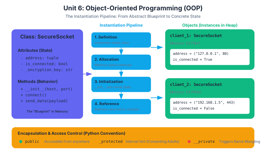
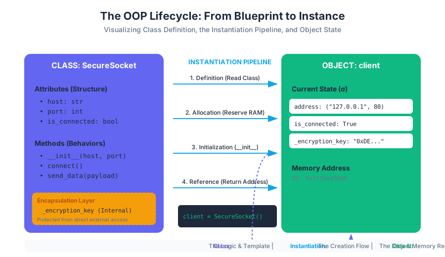
Curriculum Wrap-up and Practical Design
Key concepts: Practical program design · Problem-solving · Capstone projects · Self-paced learning
A final overview of the course principles and the application of skills through capstone projects.
Curriculum Wrap-up and Practical Design
The transition from understanding syntax to architecting systems represents the most significant hurdle in a developer's journey. While early units in the Python curriculum focus on the "what" (variables, loops, and types), the Curriculum Wrap-up and Practical Design phase focuses on the "how" and "why." This stage, often referred to as the Client Challenge, requires the synthesis of discrete computational concepts into a cohesive, functional whole. It is the move from being a student of a language to a practitioner of software engineering.
The Architecture of Problem Solving
At its core, practical program design is the application of Computational Thinking. This is not merely "thinking like a computer," but rather the process of breaking down complex, often ambiguous real-world problems into a series of steps that a deterministic machine can execute.
Decomposition and Modularity
The first step in any capstone project is decomposition: the act of breaking a large system into smaller, manageable sub-problems. In Python, this is primarily achieved through Modularity. By utilizing functions and classes, a developer can isolate logic, making the code easier to test, debug, and maintain.
The Principle of Single Responsibility (SRP): A module, function, or class should have one, and only one, reason to change. In the context of a Python simulation, this means the logic for calculating population growth should be distinct from the logic that renders that data to the console.
Sequence and State
Every program is a management of State over a Sequence of time.
- State is the current value of all variables in a program at a specific moment ($t$).
- Sequence is the order in which operations mutate that state.
In complex simulations, such as modeling population dynamics or economic shifts, managing state transitions becomes the primary challenge. If the state is mutated inconsistently (e.g., updating a list while iterating over it), the program enters an undefined or erroneous state.
Practical Program Design Patterns
When moving to open-ended projects, senior engineers rely on established patterns to avoid "spaghetti code." The following table outlines the primary design patterns introduced in the final curriculum stages.
| Pattern | Description | Primary Use Case | Python Implementation |
|---|---|---|---|
| The Accumulator | Initializing a variable and updating it within a loop. | Summing values, building strings, or filtering lists. | total += value |
| The Game Loop | A continuous while loop that processes input, updates state, and renders output. |
Interactive games and real-time simulations. | while running: update() |
| Encapsulation | Bundling data (attributes) and methods that operate on that data within a class. | Modeling real-world entities (e.g., a "Bank Account" or "Player"). | class Player: |
| The Factory | A function or method dedicated to creating and returning new objects. | Generating NPCs in a game or data points in a simulation. | def create_enemy(): |
Worked Example: The Simulation Engine
To illustrate these concepts, consider a low-level implementation of a biological simulation. This requires managing a collection of objects, iterating through time steps, and handling state mutations based on conditional logic.
import random

class Organism:
    """Represents a single entity in the simulation with state and behavior."""
    def __init__(self, species, energy):
        self.species = species
        self.energy = energy
        self.is_alive = True

    def consume(self, amount):
        """Mutates state based on external input."""
        self.energy += amount
        print(f"{self.species} consumed {amount} units. Energy: {self.energy}")

    def age(self, decay_rate):
        """Simulates the passage of time on the entity's state."""
        self.energy -= decay_rate
        if self.energy <= 0:
            self.is_alive = False

class Environment:
    """Manages the collection of organisms and the simulation loop."""
    def __init__(self, initial_pop):
        self.population = [Organism("Type-A", random.randint(10, 20)) for _ in range(initial_pop)]
        self.cycle_count = 0

    def run_cycle(self):
        """The core simulation logic (Sequence and State mutation)."""
        self.cycle_count += 1
        print(f"--- Cycle {self.cycle_count} ---")

        # Use a list comprehension to filter state (The Filter Pattern)
        self.population = [org for org in self.population if org.is_alive]

        for org in self.population:
            org.consume(random.randint(0, 5))
            org.age(decay_rate=3)

        return len(self.population) > 0

# Execution logic
sim = Environment(5)
active = True
while active:
    active = sim.run_cycle()
Algorithmic Logic and Control Flow
The "Client Challenge" often involves designing algorithms that simulate phenomena. This requires a deep understanding of Selection (if-else) and Iteration (loops).
Discrete-Time Simulations
In a simulation, we represent continuous time as a series of discrete "ticks." Mathematically, we can express the state of a system $S$ at time $t+1$ as a function of its state at time $t$:
$$S_{t+1} = f(S_t, \Delta t)$$
Where $f$ is the algorithm containing our conditional logic and arithmetic operators.
ALGORITHM: Population_Simulation
INPUT: initial_population, growth_rate, carrying_capacity, steps
OUTPUT: population_history

1. SET current_pop = initial_population
2. SET history = [current_pop]
3. FOR each step from 1 to steps:
    a. CALCULATE growth = current_pop * growth_rate * (1 - current_pop / carrying_capacity)
    b. UPDATE current_pop = current_pop + growth
    c. IF current_pop < 0 THEN SET current_pop = 0
    d. APPEND current_pop TO history
4. RETURN history
Common Mistakes in Loop Design
- Infinite Loops: Failing to update the control variable in a
whileloop, causing the program to hang. - Off-by-One Errors: Misunderstanding the
range(start, stop)function, wherestopis exclusive. - Mutation During Iteration: Modifying a list (adding/removing items) while iterating over it with a
forloop, which leads to skipped elements.
Data Structure Selection
A critical component of practical design is choosing the right tool for the job. In Python, the choice between a List and a Dictionary (or a custom Class) dictates the efficiency and readability of the solution.
| Feature | List ([]) |
Dictionary ({}) |
Class (class) |
|---|---|---|---|
| Access Method | Index (Integer) | Key (Hashable) | Attribute (Name) |
| Order | Preserved | Preserved (Python 3.7+) | N/A |
| Best For | Ordered sequences, stacks, queues. | Lookups, mapping unique keys to values. | Complex entities with state and behavior. |
| Complexity (Access) | $O(1)$ for index, $O(n)$ for value. | $O(1)$ average case. | $O(1)$ for attribute access. |
The Accumulator Pattern with Dictionaries
When processing large datasets (e.g., a list of words in a book), the dictionary is the most efficient structure for counting occurrences.
# Real-world usage: Frequency Analysis
data_stream = ["apple", "banana", "apple", "orange", "banana", "apple"]
frequency_map = {}

for item in data_stream:
    # The 'get' method allows for a default value if the key doesn't exist
    frequency_map[item] = frequency_map.get(item, 0) + 1

print(f"Final Counts: {frequency_map}")
Capstone Project Framework: From Concept to Code
The final units of the curriculum culminate in Capstone Projects. These are open-ended challenges that mirror real-world software requirements. Whether building a text-based adventure game or a data visualization tool, the workflow remains consistent.
Step 1: Requirements Gathering
Define what the program must do. For a "Client Challenge," this often involves interpreting a prompt like: "Create a system that tracks student grades and identifies those at risk of failing."
Step 2: System Design (The Blueprint)
Before writing code, map out the data structures and functions.
- Data: Will I use a list of dictionaries or a list of objects?
- Logic: What functions are needed?
calculate_average(),add_student(),generate_report().
Step 3: Implementation (The Build)
Start with a Minimum Viable Product (MVP). Get the core loop running before adding "polish" like fancy formatting or complex error handling.
Step 4: Testing and Debugging
Testing is the process of verifying that the code behaves as expected under various conditions, including "edge cases" (inputs at the extreme ends of the valid range).
Debugging and Defensive Programming
Errors are an inevitable part of the design process. Professional developers categorize these into three types:
- Syntax Errors: The "grammar" of the code is wrong (e.g., missing a colon). The program won't run at all.
- Runtime Errors: The code is valid, but something impossible happens during execution (e.g.,
ZeroDivisionErrororIndexError). - Logic Errors: The program runs without crashing, but the output is incorrect. These are the hardest to find.
Defensive Programming with Try-Except
To build robust applications, developers use Exception Handling to catch potential runtime errors before they crash the program.
# Example: Setting up a project environment for a Capstone
mkdir my_python_project
cd my_python_project
python3 -m venv venv
source venv/bin/activate  # On Windows: venv\Scripts\activate
pip install requests      # Example of adding external capabilities
touch main.py
Unit Testing Logic
Using the assert statement or the unittest library allows developers to automate the verification of their logic.
def calculate_tax(price, rate):
    if price < 0 or rate < 0:
        raise ValueError("Price and rate must be non-negative")
    return round(price * rate, 2)

# Unit Test Cases
def test_calculate_tax():
    # Standard case
    assert calculate_tax(100, 0.05) == 5.0
    # Edge case: Zero
    assert calculate_tax(0, 0.05) == 0.0
    # Edge case: Rounding
    assert calculate_tax(10.99, 0.07) == 0.77
    print("All tests passed!")

try:
    test_calculate_tax()
except AssertionError:
    print("Logic Error detected in calculate_tax")
except ValueError as e:
    print(f"Validation Error: {e}")
Self-Paced Learning and Resource Management
The final stage of the curriculum is not just about finishing the code; it's about learning how to learn. In a self-paced environment, the ability to utilize resources is a core competency.
- Solution Keys: Used not for copying, but for reverse-engineering. If a learner is stuck, they should look at the solution, understand the logic, and then attempt to implement it from scratch without looking.
- Quickstart Guides: These provide the "scaffolding" for projects, allowing learners to focus on the logic rather than the boilerplate code.
- Documentation: Learning to read the official Python documentation (docs.python.org) is the "graduation" point for any beginner.
Theorem of Independent Problem Solving: The growth of a programmer is directly proportional to the time spent in the "struggle phase"—the period between identifying a bug and finding its solution without external intervention.
Conclusion: The Path Forward
The "Curriculum Wrap-up" marks the end of guided instruction and the beginning of independent engineering. By mastering the synthesis of variables, logic, loops, and objects, the learner has transitioned from understanding how a computer works to knowing how to make a computer work for them. The final capstone projects are not just assignments; they are the first entries in a professional portfolio.
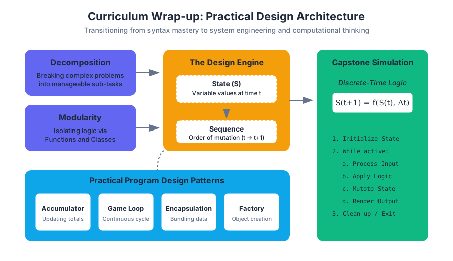
Source Materials
Study Intro to Python Fundamentals with AI — Free on Lykke
Sign up for free to generate personalized flashcards, quizzes, and study guides from this course. Chat with an AI tutor that knows the material.
Get Started FreeView this course wiki on Lykke · Browse all public course wikis