From the free course Finance Theory I on Lykke
Foundations of Finance and Time Value of Money
Key concepts: Present Value (PV) · Net Present Value (NPV) · Perpetuities and Annuities · Compounding Conventions · Leverage Ratio
Introduction to the fundamental principles of financial valuation, focusing on the time value of money and cash flow analysis.
Foundations of Finance and Time Value of Money
Overview
This section establishes the bedrock of financial theory: the axiom that a dollar today is worth more than a dollar tomorrow. This is not merely a rule of thumb but a mathematical necessity derived from the opportunity cost of capital. In this module, we move beyond simple accounting to financial economics, introducing the tools required to value sequences of cash flows across time and under conditions of certainty. We will explore how to collapse a complex future into a single, comparable number today.
AI_SVGI_SVG## Key Concepts
- Present Value (PV) & Net Present Value (NPV): The core metrics for determining the current worth of future cash flows. NPV is the primary tool for decision-making, representing the difference between the present value of cash inflows and outflows.
- Perpetuities and Annuities: Specialized formulas for valuing constant cash flows that continue forever (perpetuities) or for a fixed period (annuities).
- Compounding Conventions: Understanding how interest rates are applied over different frequencies (annual, semi-annual, continuous) and the calculation of the Effective Annual Rate (EAR).
- Leverage Ratio: An introduction to how debt influences financial positions and returns, acting as a multiplier for both gains and losses.
### Present Value (PV) and the Discount Factor
What it is
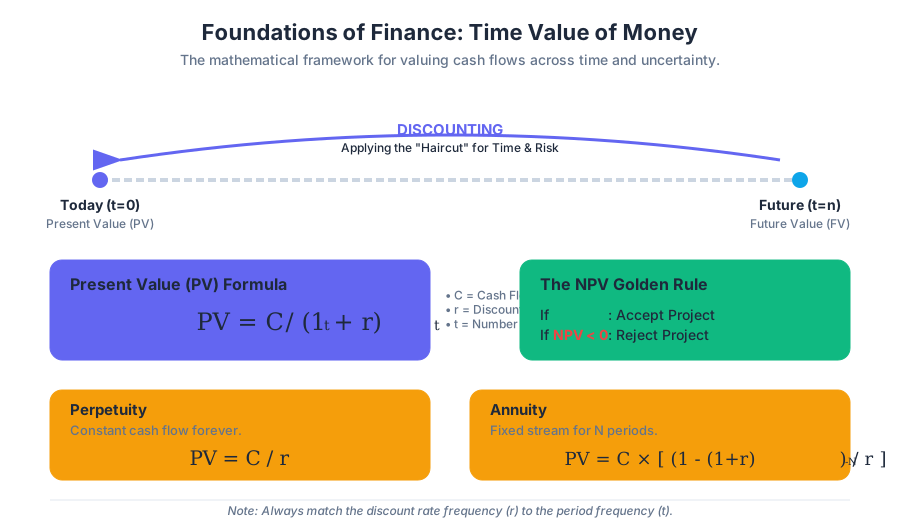
Present Value (PV) is the current value of a future sum of money or stream of cash flows given a specified rate of return. It represents the amount of money that would need to be invested today, at a given interest rate, to generate that future amount.
Mathematically, for a single cash flow $C_t$ occurring at time $t$, the Present Value is: $$PV = \frac{C_t}{(1+r)^t}$$ Where:
- $C_t$ = Cash flow at time $t$
- $r$ = Discount rate (opportunity cost of capital)
- $t$ = Number of periods
Why it matters
The PV formula is the "universal translator" of finance. It allows us to compare cash flows that occur at different points in time by bringing them all to a common denominator: "today's dollars." Without PV, we cannot objectively compare a $1,000 payment today versus a $1,200 payment in three years.
How it works: The Discount Factor
We often define the Discount Factor (DF) as the present value of $1 received at time $t$: $$DF_t = \frac{1}{(1+r)^t}$$ The discount factor is always less than 1 (assuming positive interest rates), reflecting the "haircut" we apply to future money to account for the time value.
Concrete Example
Suppose you are promised $5,000 in 3 years. If the prevailing market interest rate for an investment of similar risk is 6%, what is this promise worth today?
- $C_3 = 5,000$
- $r = 0.06$
- $t = 3$ $$PV = \frac{5,000}{(1.06)^3} = \frac{5,000}{1.191016} \approx \text{\textdollar}4,198.10$$
Common Pitfalls
- Mismatched Rates and Periods: If the cash flow occurs in 6 months, but the rate $r$ is annual, you must adjust $t$ to 0.5 or convert $r$ to a semi-annual rate.
- Ignoring Risk: The discount rate $r$ must reflect the risk of the cash flow. Using a risk-free rate for a high-risk startup investment will lead to a massive overvaluation.
### Net Present Value (NPV): The Golden Rule of Decision Making
What it is
Net Present Value (NPV) is the sum of the present values of all cash flows (both positive and negative) associated with an investment or project. It measures the net wealth created by an investment.
$$NPV = -C_0 + \sum_{t=1}^{T} \frac{C_t}{(1+r)^t}$$ Where $C_0$ is the initial investment (outlay).
Why it matters
NPV is the "Gold Standard" for capital budgeting. Unlike other metrics like the Internal Rate of Return (IRR) or Payback Period, NPV directly measures the expected increase in shareholder wealth.
The NPV Rule: Accept all projects with a positive NPV ($NPV > 0$) and reject those with a negative NPV. If comparing mutually exclusive projects, choose the one with the highest NPV.
Comparison of Decision Metrics
| Metric | Definition | Decision Rule | Major Flaw |
|---|---|---|---|
| NPV | Present value of all net cash flows | Accept if $> 0$ | Requires accurate $r$ estimation |
| IRR | The rate $r$ where $NPV = 0$ | Accept if $IRR >$ cost of cap | Can have multiple solutions; ignores scale |
| Payback | Time to recover initial outlay | Accept if $< X$ years | Ignores TVM and cash flows after payback |
| Profitability Index | Ratio of PV of inflows to Outlay | Accept if $> 1$ | Can fail when choosing between mutually exclusive projects |
Concrete Example
A company is considering a machine that costs $100,000 today ($C_0$). It is expected to generate $40,000 per year for 3 years. The discount rate is 10%.
- $PV(C_1) = 40,000 / 1.10 = 36,363.64$
- $PV(C_2) = 40,000 / 1.10^2 = 33,057.85$
- $PV(C_3) = 40,000 / 1.10^3 = 30,052.59$
- $Sum\ of\ PVs = 99,474.08$
- $NPV = 99,474.08 - 100,000 = -\text{\textdollar}525.92$ Decision: Reject the project. It destroys $525.92 of value.
### Perpetuities and Annuities
In many financial applications, we deal with constant streams of cash flows. Rather than discounting each flow individually, we use closed-form mathematical shortcuts.
1. Perpetuities
A Perpetuity is a constant stream of cash flows ($C$) that continues forever. Formula: $$PV_{perpetuity} = \frac{C}{r}$$ Derivation: This is the limit of a geometric series $\sum_{t=1}^{\infty} \frac{C}{(1+r)^t}$. As $t \to \infty$, the sum converges to $C/r$.
2. Growing Perpetuities
If the cash flow grows at a constant rate $g$ forever: $$PV_{growing\ perpetuity} = \frac{C_1}{r - g}$$ Constraint: $r$ must be greater than $g$. If $g \ge r$, the value is infinite.
3. Annuities
An Annuity is a stream of $N$ equal cash flows $C$ paid at regular intervals for a fixed period. Formula: $$PV_{annuity} = C \times \left[ \frac{1}{r} - \frac{1}{r(1+r)^N} \right]$$ The term in the brackets is often called the Annuity Factor.
4. Growing Annuities
A stream of $N$ cash flows growing at rate $g$: $$PV_{growing\ annuity} = \frac{C_1}{r-g} \left[ 1 - \left( \frac{1+g}{1+r} \right)^N \right]$$
Comparison of Stream Types
| Type | Cash Flow Pattern | Duration | Primary Use Case |
|---|---|---|---|
| Level Perpetuity | $C, C, C, ...$ | Infinite | Preferred stock, Consols |
| Growing Perpetuity | $C, C(1+g), ...$ | Infinite | Dividend Discount Model (Mature firms) |
| Level Annuity | $C, C, ...$ | $N$ periods | Mortgages, Car loans, Lease payments |
| Growing Annuity | $C, C(1+g), ...$ | $N$ periods | Retirement savings with salary growth |
AI_DEMOI_DEMO--
### Compounding Conventions and EAR
What it is
Interest rates are rarely as simple as "10% per year." The frequency with which interest is calculated (compounding) significantly changes the actual interest paid or earned.
- Annual Percentage Rate (APR): The "stated" or "nominal" rate. It does not account for compounding within the year.
- Effective Annual Rate (EAR): The actual rate earned/paid after accounting for compounding.
The Formula
To convert an APR to an EAR with $m$ compounding periods per year: $$EAR = \left( 1 + \frac{APR}{m} \right)^m - 1$$
Continuous Compounding
As $m$ approaches infinity, we reach Continuous Compounding. This is used extensively in derivatives pricing (e.g., Black-Scholes). $$EAR = e^{APR} - 1$$ $$PV = C_t \times e^{-rt}$$
Compounding Frequency Comparison (Stated Rate = 10%)
| Frequency | $m$ | Formula | EAR |
|---|---|---|---|
| Annual | 1 | $(1 + 0.10/1)^1 - 1$ | 10.00% |
| Semi-Annual | 2 | $(1 + 0.10/2)^2 - 1$ | 10.25% |
| Quarterly | 4 | $(1 + 0.10/4)^4 - 1$ | 10.38% |
| Monthly | 12 | $(1 + 0.10/12)^{12} - 1$ | 10.47% |
| Daily | 365 | $(1 + 0.10/365)^{365} - 1$ | 10.516% |
| Continuous | $\infty$ | $e^{0.10} - 1$ | 10.517% |
Implementation in Code
The following Python snippet demonstrates how to calculate NPV and compare EAR across different frequencies.
import math

def calculate_ear(apr, m=None, continuous=False):
    """Calculates Effective Annual Rate."""
    if continuous:
        return math.exp(apr) - 1
    return (1 + apr / m)**m - 1

def calculate_npv(rate, cash_flows):
    """Calculates Net Present Value for a list of cash flows."""
    return sum(cf / (1 + rate)**t for t, cf in enumerate(cash_flows))

# Example Usage
stated_rate = 0.08
flows = [-1000, 400, 400, 400] # Initial outlay of 1000, 3 years of 400

print(f"EAR (Monthly): {calculate_ear(stated_rate, m=12):.4%}")
print(f"EAR (Continuous): {calculate_ear(stated_rate, continuous=True):.4%}")
print(f"Project NPV: ${calculate_npv(stated_rate, flows):.2f}")
### Leverage Ratio
What it is
Leverage refers to the use of borrowed money (debt) to finance the purchase of assets, with the expectation that the income or capital gain from the new asset will exceed the cost of borrowing.
The Leverage Ratio can be defined in several ways, but a common version is: $$Leverage = \frac{Total\ Assets}{Equity}$$ Or the Debt-to-Equity Ratio: $$D/E = \frac{Total\ Debt}{Total\ Equity}$$
Why it matters
Leverage is a double-edged sword. It magnifies the Return on Equity (ROE). If the return on assets (ROA) is higher than the interest rate on debt, leverage increases ROE. If ROA is lower than the interest rate, leverage accelerates losses.
How it works: The ROE Formula
$$ROE = \frac{Net\ Income}{Equity} = [ROA + (ROA - Interest\ Rate) \times \frac{Debt}{Equity}] \times (1 - Tax\ Rate)$$
Concrete Example: The Power of Leverage
Imagine two investors, A and B, both buying a $1,000,000 building.
- Investor A (No Leverage): Pays $1M cash.
- Investor B (Leveraged): Pays $200k cash (Equity) and borrows $800k at 5% interest.
Scenario: Building value increases by 10% ($100k gain)
- Investor A: $100k gain on $1M investment = 10% Return.
- Investor B: $100k gain - $40k interest = $60k profit. $60k profit on $200k investment = 30% Return.
Scenario: Building value decreases by 10% ($100k loss)
- Investor A: $100k loss on $1M investment = -10% Return.
- Investor B: $100k loss + $40k interest = $140k total loss. $140k loss on $200k investment = -70% Return.
Common Pitfalls
- Ignoring the Cost of Financial Distress: High leverage increases the probability of bankruptcy. The "cost" of leverage isn't just the interest rate; it's the risk of total loss.
- Volatility Miscalculation: Investors often underestimate how quickly a small dip in asset prices can wipe out equity when leverage is 10x or 20x (common in pre-2008 investment banking).
AI_FLASHCARDSI_FLASHCARDS Present Value (PV): $PV = C / (1+r)^t$
- Net Present Value (NPV): Sum of all discounted cash flows; $NPV > 0$ means value creation.
- Perpetuity: $PV = C / r$
- Annuity Factor: $[1/r - 1/(r(1+r)^N)]$
- EAR (Periodic): $(1 + APR/m)^m - 1$
- EAR (Continuous): $e^{APR} - 1$
- Leverage Ratio: Total Assets / Equity; magnifies both risk and reward.
- Opportunity Cost of Capital: The expected return foregone by investing in a project rather than in comparable financial securities.
AI_QUIZI_QUIZ. Scenario: You are offered a choice between $10,000 today or $11,000 in one year. If the market interest rate is 12%, which should you choose?
- Answer: Choose $10,000 today. The PV of $11,000 is $11,000 / 1.12 = $9,821.43, which is less than $10,000.
- Concept: Why does the NPV rule dominate the IRR rule for mutually exclusive projects of different scales?
- Answer: Because IRR is a percentage and doesn't account for the absolute dollar value created. A 100% return on $1 is worse than a 10% return on $1,000,000.
- Calculation: If a bank quotes an APR of 12% compounded monthly, what is the EAR?
- Answer: $(1 + 0.12/12)^{12} - 1 = (1.01)^{12} - 1 \approx 12.68%$.
- Theory: What happens to the PV of an annuity if the interest rate $r$ increases?
- Answer: The PV decreases. Since $r$ is in the denominator of the discount factor, a higher $r$ reduces the value of future cash flows.
- Leverage: If a firm has a Debt-to-Equity ratio of 1.0 and its ROA is 8% while its interest rate is 5%, what is its ROE (ignoring taxes)?
- Answer: $ROE = 8% + (8% - 5%) \times 1.0 = 11%$.
AI_STUDY_GUIDEI_STUDY_GUIDE## Study Guide: Foundations of Finance
1. Fundamental Principles
- Time Value of Money (TVM): Understand that the value of money is a function of time, risk, and opportunity cost.
- The Law of One Price: In efficient markets, two assets with the same cash flows must have the same price. This underlies all PV calculations.
2. Mathematical Mastery
- Practice converting between APR and EAR. This is a frequent source of error in exams and professional modeling.
- Memorize the Annuity and Perpetuity formulas. You should be able to derive the perpetuity formula using the sum of a geometric series.
- Understand the Relationship between $r$ and $PV$: They are inversely related. Understand the relationship between $t$ and $PV$: They are also inversely related.
3. Decision Criteria
- Be able to calculate NPV for uneven cash flow streams.
- Explain why NPV is the superior decision metric compared to Payback, IRR, and Book Rate of Return.
- Know the conditions under which IRR fails (e.g., non-conventional cash flows, mutually exclusive projects).
4. Leverage and Risk
- Understand the Balance Sheet identity: $Assets = Liabilities + Equity$.
- Be able to calculate the impact of Leverage on ROE.
- Recognize that leverage does not create value in a frictionless world (Modigliani-Miller), but it changes the risk profile of the equity holders.
5. Real-World Applications
- Bond Pricing: A bond is simply an annuity (coupons) plus a single payment (par value).
- Stock Valuation: A stock can be modeled as a growing perpetuity of dividends.
- Mortgages: An amortizing loan is a level annuity.
Source Materials
Study Finance Theory I on Lykke
This course page is free to open: signed out, you can read its first two sections, and signing in, on any plan, opens the rest. The free Lykke Chrome extension syncs your own Canvas courses, so ChatGPT, Claude and Muse can answer from your classes and deadlines. It only reads Canvas.
Add the free extensionSign in to open every section