From the free course Finance Theory I on Lykke
Fixed-Income Securities
Key concepts: Coupon Bonds · Yield Curves · Spot and Forward Rates · Modified Duration · Law of One Price
Exploration of bond valuation, interest rate dynamics, and the term structure of interest rates.
Fixed-Income Securities
Fixed-income securities represent the bedrock of the global financial system. While equity markets often capture the public imagination, the fixed-income market—comprising government debt, corporate bonds, and securitized products—is significantly larger in terms of total notional value and serves as the primary mechanism for capital allocation and monetary policy transmission.
In this section, we move beyond the basic time-value-of-money (TVM) principles to explore the rigorous mechanics of debt instruments. We will define how these securities are priced, how their risks are quantified through duration and convexity, and how the "term structure" of interest rates provides a window into the market's collective expectation of the future.
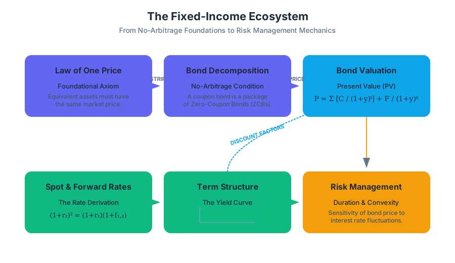
AI_SVGI_SVGThe Fixed-Income Ecosystem: A visualization showing the flow from the Law of One Price to Spot/Forward rates, leading to Bond Valuation and finally to Risk Management via Duration and Convexity.*
The Law of One Price and No-Arbitrage
The foundational axiom of modern finance is the Law of One Price (LoOP). It states that in a competitive market, if two assets are equivalent in all relevant aspects (specifically their cash flow timing and risk profile), they must have the same market price.
In the context of fixed-income, this implies that a complex security, such as a coupon-bearing bond, can be viewed as a "package" of simpler securities. Specifically, any bond can be decomposed into a series of Zero-Coupon Bonds (ZCBs).
Theorem: The No-Arbitrage Condition If a coupon bond provides cash flows $C_1, C_2, \dots, C_n$ at times $t_1, t_2, \dots, t_n$, and the market price of a ZCB maturing at time $t$ is $P(0, t)$, then the price of the coupon bond $P_{bond}$ must satisfy: $$P_{bond} = \sum_{i=1}^{n} C_i \cdot P(0, t_i)$$ If $P_{bond}$ were higher, an arbitrageur would sell the bond and buy the individual ZCBs (strips) to lock in a riskless profit. If lower, they would do the reverse.
Implications for Valuation
This principle allows us to value any fixed-income instrument without needing a single "interest rate." Instead, we use the specific discount factor relevant to each specific maturity.
Coupon Bonds: Mechanics and Valuation
A Coupon Bond is a debt instrument where the issuer (borrower) commits to making periodic interest payments (coupons) and returning the face value (principal) at maturity.
The Valuation Formula
The price of a bond is the present value (PV) of its future cash flows, discounted at the Yield to Maturity (YTM), denoted as $y$. For a bond with face value $F$, annual coupon rate $c$, and $n$ periods to maturity:
$$P = \sum_{t=1}^{n} \frac{C}{(1+y)^t} + \frac{F}{(1+y)^n}$$
Where $C = \frac{c \cdot F}{m}$ (if payments are $m$ times per year).
Bond Price Dynamics
The relationship between a bond's coupon rate and its YTM determines whether it trades at a premium or a discount.
| Relationship | Bond Status | Price vs. Face Value |
|---|---|---|
| Coupon Rate > YTM | Premium | $P > F$ |
| Coupon Rate < YTM | Discount | $P < F$ |
| Coupon Rate = YTM | Par | $P = F$ |
Worked Example: Pricing a Semi-Annual Bond
Consider a corporate bond with:
- Face Value ($F$): $1,000
- Coupon Rate: 6% (paid semi-annually)
- Maturity: 2 years
- YTM: 4% (annualized)
Step 1: Identify Parameters
- $C = (0.06 \times 1000) / 2 = \text{\textdollar}30$
- $n = 2 \times 2 = 4$ periods
- $y_{period} = 0.04 / 2 = 0.02$ (2%)
Step 2: Calculate PV $$P = \frac{30}{(1.02)^1} + \frac{30}{(1.02)^2} + \frac{30}{(1.02)^3} + \frac{1030}{(1.02)^4}$$ $$P = 29.41 + 28.83 + 28.27 + 951.55 = \text{\textdollar}1,038.06$$ The bond trades at a premium because the coupon (6%) is higher than the market required return (4%).
The Term Structure of Interest Rates
The Term Structure describes the relationship between interest rates and the time to maturity for a given class of bonds (usually risk-free government bonds). This is visualized through the Yield Curve.
Spot Rates vs. Forward Rates
To understand the term structure, we must distinguish between different types of rates:
- Spot Rate ($r_t$): The annualized interest rate agreed upon today for a loan that begins immediately and lasts for $t$ periods.
- Forward Rate ($f_{t, T}$): The interest rate agreed upon today for a loan that will begin at a future date $t$ and end at date $T$.
The Forward Rate Derivation
Under the No-Arbitrage assumption, the return from investing in a long-term spot contract must equal the return from rolling over a series of short-term contracts.
For a two-period horizon: $$(1 + r_2)^2 = (1 + r_1)(1 + f_{1,2})$$
Solving for the forward rate: $$f_{1,2} = \frac{(1 + r_2)^2}{(1 + r_1)} - 1$$
Yield Curve Theories
Why is the yield curve shaped the way it is? There are three primary economic explanations:
| Theory | Core Logic | Implications |
|---|---|---|
| Expectations Hypothesis | Long-term rates are the average of expected future short-term rates. | An upward slope means the market expects rates to rise. |
| Liquidity Preference | Investors demand a premium for the risk of locking up capital for longer periods. | The curve should naturally slope upward (Liquidity Premium). |
| Market Segmentation | Different investors (pension funds vs. banks) prefer different maturities. | Supply and demand in specific "buckets" determine the shape. |
AI_DEMOI_DEMOInteractive Yield Curve: A simulation where users can adjust inflation expectations and liquidity premiums to see how the Yield Curve shifts from Normal to Inverted.*
Interest-Rate Risk: Duration and Convexity
Bond prices move inversely to interest rates. However, not all bonds react with the same intensity. Duration is the primary metric used to quantify this sensitivity.
Macaulay Duration ($D_{mac}$)
Macaulay Duration is the weighted average time to receive the cash flows from a bond, measured in years.
$$D_{mac} = \frac{\sum_{t=1}^{n} t \cdot PV(CF_t)}{P}$$
Modified Duration ($D_{mod}$)
To find the actual percentage change in price for a given change in yield, we use Modified Duration:
$$D_{mod} = \frac{D_{mac}}{1 + y}$$
The Duration Rule: The approximate percentage change in a bond's price for a small change in yield ($\Delta y$) is: $$\frac{\Delta P}{P} \approx -D_{mod} \cdot \Delta y$$
Convexity: The Second-Order Effect
The relationship between bond prices and yields is not linear; it is convex. Duration is merely the first derivative (the slope) of the price-yield curve. For large interest rate moves, duration underestimates the price of the bond.
Convexity ($C$) accounts for the curvature. The more accurate price change formula is: $$\frac{\Delta P}{P} \approx -D_{mod} \cdot \Delta y + \frac{1}{2} C \cdot (\Delta y)^2$$
Comparison of Sensitivity Factors
| Factor | Effect on Duration | Effect on Interest Rate Risk |
|---|---|---|
| Higher Coupon | Decreases | Lower risk (capital returned faster) |
| Longer Maturity | Increases | Higher risk (more time for rates to fluctuate) |
| Higher YTM | Decreases | Lower risk (discounting dampens future CFs) |
Implementation: Bond Pricing and Risk Engine
In modern finance, these calculations are automated. Below is a high-signal Python implementation using numpy to calculate the price, Macaulay Duration, and Modified Duration of a bond.
import numpy as np

def calculate_bond_metrics(face_value, coupon_rate, ytm, years, freq=2):
    """
    Calculates Price, Macaulay Duration, and Modified Duration.
    freq: 1 for annual, 2 for semi-annual, 4 for quarterly.
    """
    periods = years * freq
    coupon_payment = (coupon_rate * face_value) / freq
    periodic_ytm = ytm / freq

    times = np.arange(1, periods + 1)
    cash_flows = np.array([coupon_payment] * (periods - 1) + [coupon_payment + face_value])

    # Discount factors: 1 / (1 + r)^t
    discount_factors = 1 / (1 + periodic_ytm)**times
    pv_cash_flows = cash_flows * discount_factors

    price = np.sum(pv_cash_flows)

    # Macaulay Duration in periods
    macaulay_duration_periods = np.sum(times * pv_cash_flows) / price
    macaulay_duration_years = macaulay_duration_periods / freq

    # Modified Duration
    modified_duration = macaulay_duration_years / (1 + periodic_ytm)

    return {
        "Price": round(price, 2),
        "Macaulay Duration": round(macaulay_duration_years, 3),
        "Modified Duration": round(modified_duration, 3)
    }

# Example: 10-year, 5% coupon bond, 4% YTM
metrics = calculate_bond_metrics(1000, 0.05, 0.04, 10)
print(metrics)
# Output: {'Price': 1081.76, 'Macaulay Duration': 7.989, 'Modified Duration': 7.832}
Common Pitfalls in Fixed-Income Analysis
- Ignoring Reinvestment Risk: The YTM calculation assumes all coupons are reinvested at the same YTM rate. In a falling-rate environment, the actual realized return will be lower than the YTM.
- Confusing Nominal and Real Rates: Fixed-income investors are highly sensitive to inflation. If nominal rates are 5% but inflation is 6%, the real return is negative.
- Duration Misapplication: Duration is only a local approximation. For large "shocks" to the yield curve (e.g., a 200 basis point move), failing to include convexity will lead to significant pricing errors.
- The "Pull to Par" Illusion: Investors often think discount bonds are "cheaper." However, the price appreciation toward par is simply a component of the YTM, not an excess return.
AI_FLASHCARDSI_FLASHCARDS Spot Rate: The yield on a zero-coupon bond for a specific maturity.
- Forward Rate: An interest rate set today for a loan occurring in the future.
- Yield to Maturity (YTM): The internal rate of return (IRR) of a bond's cash flows.
- Macaulay Duration: The weighted average time to receive cash flows.
- Modified Duration: A measure of price sensitivity to interest rate changes ($\Delta P/P$).
- Convexity: The measure of the curvature in the relationship between bond prices and yields.
- Law of One Price: The rule that identical cash flows must have identical prices.
AI_QUIZI_QUIZ. If the yield curve is inverted (short-term rates > long-term rates), what does the Expectations Hypothesis suggest about future interest rates? 2. A bond has a Modified Duration of 8.0. If interest rates rise by 50 basis points (0.50%), what is the approximate percentage change in the bond's price? 3. Why does a zero-coupon bond have a Macaulay Duration exactly equal to its maturity? 4. Between a 5% coupon bond and a 0% coupon bond, both with 10 years to maturity, which has higher interest rate risk? 5. If a bond's price is $1,050 and its face value is $1,000, is the YTM higher or lower than the coupon rate?
AI_STUDY_GUIDEI_STUDY_GUIDE*Key Formulas to Memorize:**
- Bond Price: $P = \sum \frac{C}{(1+y)^t} + \frac{F}{(1+y)^n}$
- Forward Rate (1-period): $f_{t, t+1} = \frac{(1+r_{t+1})^{t+1}}{(1+r_t)^t} - 1$
- Duration Rule: $\Delta P/P \approx -D_{mod} \cdot \Delta y$
- Modified Duration: $D_{mod} = D_{mac} / (1+y)$
Conceptual Checklist:
- Can I explain why bond prices and yields move inversely?
- Do I understand how to bootstrap a spot curve from coupon bond prices?
- Can I distinguish between the three main yield curve theories?
- Do I know when to use duration vs. when convexity is required?
- Can I apply the Law of One Price to identify an arbitrage opportunity?
Suggested Practice:
- Calculate the price of a 5-year bond with a 4% coupon when the market rate is 6%.
- Derive the 1-year forward rate starting in year 2, given spot rates $r_1=2%, r_2=3%, r_3=4%$.
- Use the Python code block above to test how changing the
freq(compounding frequency) affects the bond price.
Source Materials
Study Finance Theory I on Lykke
This course page is free to open: signed out, you can read its first two sections, and signing in, on any plan, opens the rest. The free Lykke Chrome extension syncs your own Canvas courses, so ChatGPT, Claude and Muse can answer from your classes and deadlines. It only reads Canvas.
Add the free extensionSign in to open every section