From the free course Finance Theory I on Lykke
Equity Valuation and Common Stocks
Key concepts: Dividend Discount Model (DDM) · Gordon Growth Model · Earnings-Per-Share (EPS) · Price-Earnings (P/E) Ratio · Present Value of Growth Opportunities (PVGO)
Analysis of common stocks and the models used to determine their intrinsic value based on future earnings and dividends.
Equity Valuation and Common Stocks
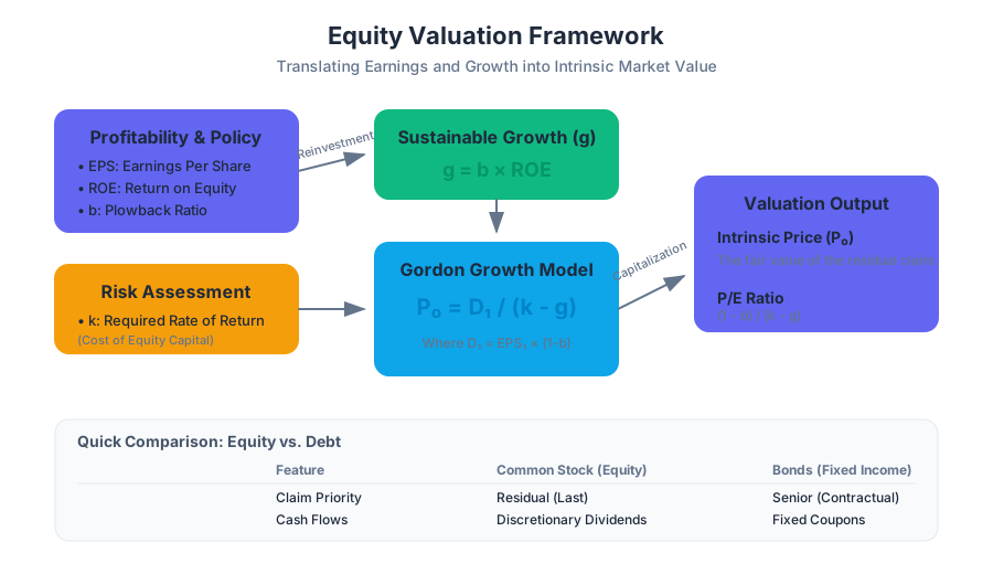
In the hierarchy of financial claims, equity represents the residual interest in the assets of an entity after deducting all its liabilities. Unlike fixed-income securities, which promise a predetermined schedule of cash flows, common stocks offer a claim on the uncertain future prosperity of a corporation. Valuing these claims requires a synthesis of accounting metrics, growth forecasts, and risk assessments.
This article explores the fundamental theoretical framework for equity valuation, moving from the foundational Dividend Discount Model (DDM) to the more nuanced Present Value of Growth Opportunities (PVGO). We will examine how market participants translate earnings and growth expectations into the price-to-earnings (P/E) multiples seen on trading screens every day.
AI_SVGI_SVG--
The Dividend Discount Model (DDM)
The Dividend Discount Model (DDM) is the bedrock of fundamental equity analysis. It posits that the intrinsic value of a share of stock is the present value of all future dividends expected to be paid by the company, discounted at an appropriate risk-adjusted rate.
1. What it is
The DDM treats a stock as a sequence of cash flows ($D_1, D_2, \dots, D_n$). Mathematically, the price today ($P_0$) is expressed as:
$$P_0 = \sum_{t=1}^{\infty} \frac{E[D_t]}{(1+k)^t}$$
Where:
- $P_0$: Current intrinsic value of the stock.
- $D_t$: Expected dividend at time $t$.
- $k$: The required rate of return (cost of equity capital).
2. Why it matters
The DDM solves the "horizon problem." While an investor might plan to sell a stock in three years, the price they receive at that time will depend on what the next investor expects to receive in dividends thereafter. By extending the horizon to infinity, we capture the total fundamental value of the enterprise without needing to guess future market sentiment at a specific exit date.
3. How it works: The Law of One Price
The model is derived from the assumption that in a competitive market, the price of an asset must equal the present value of its future payoffs. If an investor holds a stock for one year, their return comes from the dividend ($D_1$) and the capital gain ($P_1 - P_0$).
$$k = \frac{D_1 + P_1 - P_0}{P_0}$$
Rearranging for $P_0$:
$$P_0 = \frac{D_1 + P_1}{1+k}$$
By recursively substituting the expression for $P_1, P_2, \dots$, we arrive at the infinite series formula.
4. Comparison: Equity vs. Debt Valuation
| Feature | Fixed-Income (Bonds) | Common Stock (Equity) |
|---|---|---|
| Cash Flow Nature | Contractual (Coupons/Principal) | Discretionary (Dividends) |
| Maturity | Finite (usually) | Perpetual (Going concern) |
| Priority | Senior claim | Residual claim |
| Discount Rate | Yield to Maturity (YTM) | Cost of Equity ($k$) |
| Growth | Usually zero/fixed | Variable and uncertain |
The Gordon Growth Model (GGM)
While the general DDM is theoretically robust, it is practically difficult to forecast infinite individual dividends. The Gordon Growth Model (GGM), or Constant Growth Model, simplifies this by assuming dividends grow at a constant rate ($g$) forever.
1. The Formula
If dividends grow at rate $g$, then $D_t = D_0(1+g)^t$. Substituting this into the DDM formula yields a geometric series that converges to:
$$P_0 = \frac{D_1}{k - g}$$
2. Derivation (The Geometric Series Proof)
To understand why this works, consider the sum $S$: $$S = \frac{D_1}{1+k} + \frac{D_1(1+g)}{(1+k)^2} + \frac{D_1(1+g)^2}{(1+k)^3} + \dots$$
This is a geometric series with the first term $a = \frac{D_1}{1+k}$ and common ratio $r = \frac{1+g}{1+k}$. The sum of an infinite geometric series $a / (1-r)$ converges if $|r| < 1$ (which implies $k > g$).
$$P_0 = \frac{\frac{D_1}{1+k}}{1 - \frac{1+g}{1+k}} = \frac{D_1}{(1+k) - (1+g)} = \frac{D_1}{k - g}$$
3. Concrete Example
Suppose "BlueChip Corp" just paid a dividend ($D_0$) of $2.00. The expected growth rate ($g$) is 5%, and the required return ($k$) is 10%.
- Calculate $D_1$: $\text{\textdollar}2.00 \times (1 + 0.05) = \text{\textdollar}2.10$.
- Apply GGM: $P_0 = \frac{2.10}{0.10 - 0.05} = \frac{2.10}{0.05} = \text{\textdollar}42.00$.
4. Sensitivity Analysis
The GGM is highly sensitive to the inputs $k$ and $g$. As $g$ approaches $k$, the price approaches infinity.
| Growth Rate ($g$) | Required Return ($k$) | Resulting Price ($P_0$) |
|---|---|---|
| 4% | 10% | $35.00 |
| 5% | 10% | $42.00 |
| 6% | 10% | $53.00 |
| 5% | 9% | $52.50 |
5. Common Pitfalls
- $g \ge k$: If the growth rate exceeds the discount rate, the formula breaks down. In reality, no company can grow faster than the overall economy forever.
- Non-dividend payers: The GGM cannot directly value firms like Amazon or Google that reinvest all earnings (though one can argue $D_t$ represents the capacity to pay dividends).
Earnings-Per-Share (EPS) and the P/E Ratio
While dividends are the cash actually received by shareholders, Earnings-Per-Share (EPS) represents the total profit available to be either distributed or reinvested. The Price-Earnings (P/E) Ratio is the most widely used metric for relative valuation.
1. Definitions
- EPS: $\frac{\text{Total Net Income}}{\text{Shares Outstanding}}$
- Plowback Ratio ($b$): The fraction of earnings reinvested in the firm.
- Dividend Payout Ratio ($1-b$): The fraction of earnings paid out as dividends.
Therefore: $D_1 = EPS_1 \times (1-b)$.
2. The Link Between Growth and Reinvestment
A firm's growth rate is not arbitrary; it is a function of how much it reinvests and the return it earns on that reinvestment. $$g = \text{Retention Ratio} \times \text{Return on Equity (ROE)} = b \times ROE$$
3. Deriving the P/E Ratio
Starting from the GGM: $$P_0 = \frac{EPS_1(1-b)}{k - (b \times ROE)}$$
Dividing both sides by $EPS_1$: $$\frac{P_0}{EPS_1} = \frac{1-b}{k - g}$$
4. Determinants of the P/E Ratio
The P/E ratio is a reflection of three things:
- Growth opportunities: Higher $g$ leads to higher P/E.
- Risk: Higher $k$ (risk) leads to lower P/E.
- Accounting Quality: The "E" must represent true economic reality.
AI_DEMOI_DEMO--
Present Value of Growth Opportunities (PVGO)
One of the most powerful concepts in finance is the decomposition of a stock's price into two components: the value of its current assets and the value of its future growth.
1. What it is
The PVGO is the net present value of all future investments the firm will make. We can express the stock price as: $$P_0 = \frac{EPS_1}{k} + PVGO$$
Where:
- $\frac{EPS_1}{k}$: The value of the firm if it paid out all earnings as dividends (a "no-growth" firm).
- $PVGO$: The additional value created by reinvesting earnings into projects with $ROE > k$.
2. Why it matters: Growth vs. Value
A company can grow its earnings simply by reinvesting cash ($b > 0$), but this only adds value to the stock price if the return on those investments ($ROE$) exceeds the cost of capital ($k$).
- If $ROE > k$, then $PVGO > 0$ (Growth adds value).
- If $ROE = k$, then $PVGO = 0$ (Growth is value-neutral).
- If $ROE < k$, then $PVGO < 0$ (Growth destroys value).
3. Worked Example: The Growth Trap
Consider two firms, both with $EPS_1 = \text{\textdollar}5.00$ and $k = 10%$.
Firm A (High ROE): $b = 0.6$, $ROE = 15%$.
- $g = 0.6 \times 0.15 = 9%$.
- $P_0 = \frac{5(1-0.6)}{0.10 - 0.09} = \frac{2}{0.01} = \text{\textdollar}200$.
- No-growth value = $5 / 0.10 = \text{\textdollar}50$.
- $PVGO = \text{\textdollar}200 - \text{\textdollar}50 = \text{\textdollar}150$. (75% of value is growth).
Firm B (Low ROE): $b = 0.6$, $ROE = 8%$.
- $g = 0.6 \times 0.08 = 4.8%$.
- $P_0 = \frac{5(1-0.6)}{0.10 - 0.048} = \frac{2}{0.052} \approx \text{\textdollar}38.46$.
- No-growth value = $\text{\textdollar}50$.
- $PVGO = \text{\textdollar}38.46 - \text{\textdollar}50 = -\text{\textdollar}11.54$. (The firm is destroying value by reinvesting).
4. Summary Table: PVGO Dynamics
| Scenario | Condition | Impact of Increasing Plowback ($b$) | Stock Category |
|---|---|---|---|
| Value Creation | $ROE > k$ | Price Increases | Growth Stock |
| Value Neutral | $ROE = k$ | Price Unchanged | Mature/Income Stock |
| Value Destruction | $ROE < k$ | Price Decreases | "Empire Builders" |
Implementation: Multistage Valuation in Python
In the real world, companies often go through a "high growth" phase before maturing. A simple GGM is insufficient. We use a Two-Stage DDM where we discount individual dividends for the high-growth period and use a terminal value for the steady-state period.
def calculate_intrinsic_value(d0, high_g, stable_g, k, years_high_growth):
    """
    Calculates the intrinsic value of a stock using a two-stage DDM.

    d0: Current dividend
    high_g: Growth rate during high-growth phase (decimal)
    stable_g: Terminal growth rate (decimal)
    k: Required rate of return (decimal)
    years_high_growth: Duration of the first stage
    """
    pv_dividends = 0
    current_d = d0

    # Stage 1: High Growth Phase
    for t in range(1, years_high_growth + 1):
        current_d *= (1 + high_g)
        pv_dividends += current_d / ((1 + k) ** t)

    # Stage 2: Terminal Value (at the end of Stage 1)
    d_terminal = current_d * (1 + stable_g)
    terminal_price = d_terminal / (k - stable_g)
    pv_terminal_value = terminal_price / ((1 + k) ** years_high_growth)

    intrinsic_value = pv_dividends + pv_terminal_value
    return round(intrinsic_value, 2)

# Example: Tech startup transitioning to maturity
# $1.00 dividend, 20% growth for 5 years, then 4% stable growth. 10% discount rate.
price = calculate_intrinsic_value(1.00, 0.20, 0.04, 0.10, 5)
print(f"The intrinsic value is: ${price}")
# Output: The intrinsic value is: $34.58
Variations and Extensions
1. The H-Model
The H-model is a variation of the two-stage DDM that assumes the growth rate does not drop abruptly but rather declines linearly from a high initial rate to a stable terminal rate. This is often more realistic for firms facing increasing competition.
2. Free Cash Flow to Equity (FCFE)
For firms that do not pay dividends, analysts often substitute "Dividends" with FCFE, which is the cash flow available to be paid out after all reinvestment needs and debt obligations are met. $$FCFE = \text{Net Income} + \text{Depreciation} - \text{CapEx} - \Delta\text{Working Capital} + \text{Net Borrowing}$$
3. The Fed Model
The Fed Model compares the earnings yield ($E/P$) of the S&P 500 to the yield on 10-year Treasury bonds. While popular, it is often criticized for comparing a real variable (earnings, which grow with inflation) to a nominal variable (bond yields).
Common Pitfalls in Equity Valuation
- Double Counting Growth: Beginners often include growth in the cash flow projections and use a high P/E ratio for the terminal value. The terminal P/E should reflect a mature, stable-growth company.
- Ignoring Risk in $k$: Using a single discount rate for all companies. A biotech startup requires a significantly higher $k$ than a utility company due to the variance of its cash flows.
- The "Low P/E" Trap: Assuming a low P/E stock is "cheap." A low P/E might be a rational market response to a company with $ROE < k$ or a business model facing obsolescence.
- Terminal Value Dominance: In many DCF models, the terminal value accounts for 70-90% of the total price. Small changes in the terminal growth rate ($g$) can lead to massive swings in valuation, making the model appear more precise than it actually is.
Source Materials
Study Finance Theory I on Lykke
This course page is free to open: signed out, you can read its first two sections, and signing in, on any plan, opens the rest. The free Lykke Chrome extension syncs your own Canvas courses, so ChatGPT, Claude and Muse can answer from your classes and deadlines. It only reads Canvas.
Add the free extensionSign in to open every section