From the free course Finance Theory I on Lykke
Asset Pricing Models: CAPM and APT
Key concepts: Capital Asset Pricing Model (CAPM) · Beta (β) · Security Market Line (SML) · Arbitrage Pricing Theory (APT) · Systematic vs. Idiosyncratic Risk
Examination of equilibrium models that determine the required rate of return for risky assets.
Asset Pricing Models: CAPM and APT
In the trajectory of modern finance, the transition from Markowitz’s Portfolio Selection—which focuses on how an individual should invest—to Asset Pricing Models represents a shift from normative behavior to positive equilibrium. If Portfolio Theory tells us how to construct the "best" portfolio, Asset Pricing Models like the Capital Asset Pricing Model (CAPM) and Arbitrage Pricing Theory (APT) explain how the collective actions of all investors result in the prices and expected returns we observe in the marketplace.
These models serve as the foundational "hurdle rate" logic in corporate finance. Whether a CFO is deciding on a multi-billion dollar capital expenditure or a fund manager is evaluating a tech IPO, they are using the mathematical frameworks derived from CAPM and APT to determine if the expected return justifies the inherent risk.
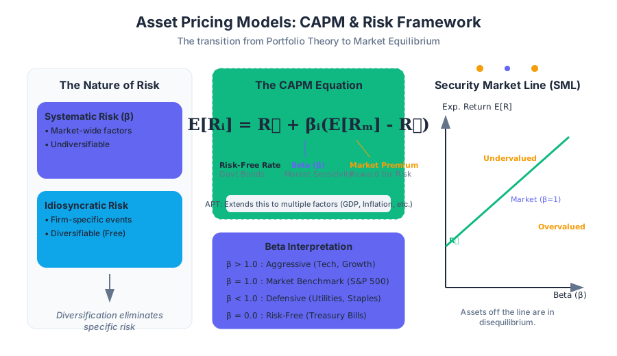
AI_SVGI_SVG## The Fundamental Dichotomy: Systematic vs. Idiosyncratic Risk
Before deriving specific models, we must establish the two-part nature of risk. In a diversified economy, not all uncertainty is created equal.
- Systematic Risk (Market Risk): This refers to fluctuations that affect the entire market simultaneously. Examples include changes in GDP, interest rate hikes, or global pandemics. Because these factors impact all firms to varying degrees, this risk cannot be diversified away.
- Idiosyncratic Risk (Specific Risk): This refers to risks unique to a specific company or industry, such as a CEO resignation, a localized factory fire, or a successful patent application. In a large enough portfolio, these "shocks" cancel each other out.
The Diversification Principle: In a competitive market, investors are not compensated for bearing idiosyncratic risk. Because this risk can be eliminated for free (via diversification), the market price of idiosyncratic risk is zero. Only systematic risk commands a risk premium.
| Feature | Systematic Risk | Idiosyncratic Risk |
|---|---|---|
| Synonyms | Market Risk, Undiversifiable Risk | Firm-Specific Risk, Unique Risk |
| Source | Macroeconomic factors (Inflation, GDP) | Microeconomic factors (Strikes, R&D) |
| Remedy | Hedging / Asset Allocation | Diversification |
| Market Reward | Yes (Risk Premium) | No |
The Capital Asset Pricing Model (CAPM)
Developed independently by Sharpe (1964), Lintner (1965), and Mossin (1966), the CAPM is a linear model that predicts the expected return of an asset based on its sensitivity to the broad market.
The Assumptions of CAPM
To arrive at the elegant simplicity of the CAPM, we assume a "frictionless" world:
- Rationality: Investors are mean-variance optimizers.
- Homogeneous Expectations: All investors have the same estimates of expected returns, variances, and covariances.
- Single-Period Horizon: All investors plan for the same time duration.
- Perfect Markets: No taxes, no transaction costs, and assets are infinitely divisible.
- Risk-Free Rate: Investors can borrow and lend at the same risk-free rate ($R_f$).
The CAPM Formula
The expected return of any asset $i$ is defined as:
$$E[R_i] = R_f + \beta_i (E[R_m] - R_f)$$
Where:
- $E[R_i]$: Expected return on asset $i$.
- $R_f$: The risk-free rate (typically long-term government bond yields).
- $\beta_i$: The asset's Beta, measuring systematic risk.
- $E[R_m] - R_f$: The Equity Market Risk Premium (EMRP), the extra return required for moving from a risk-free asset to the risky market portfolio.
Beta (β): The Measure of Sensitivity
Beta is the most critical parameter in the CAPM. It represents the marginal contribution of an asset to the risk of the market portfolio. Mathematically, it is the ratio of the covariance between the asset and the market to the variance of the market:
$$\beta_i = \frac{Cov(R_i, R_m)}{Var(R_m)} = \rho_{im} \frac{\sigma_i}{\sigma_m}$$
Where $\rho_{im}$ is the correlation between the asset and the market.
Interpreting Beta Values
- $\beta = 1$: The asset moves in lockstep with the market. If the market rises 10%, the asset is expected to rise 10%.
- $\beta > 1$: "Aggressive" assets. These are more sensitive to market swings (e.g., high-growth tech stocks).
- $0 < \beta < 1$: "Defensive" assets. These move less than the market (e.g., utility companies).
- $\beta = 0$: The asset has no systematic risk (e.g., the risk-free asset).
- $\beta < 0$: The asset moves inversely to the market (extremely rare, sometimes seen in gold or specific hedging instruments).
| Asset Class | Typical Beta Range | Sensitivity Description |
|---|---|---|
| Treasury Bills | 0.0 | No market sensitivity |
| Utilities | 0.4 – 0.7 | Low sensitivity; "Defensive" |
| S&P 500 Index | 1.0 | The Market Benchmark |
| Tech / Biotech | 1.2 – 2.5 | High sensitivity; "Aggressive" |
The Security Market Line (SML)
The Security Market Line is the graphical representation of the CAPM. It plots the relationship between an asset's Beta (x-axis) and its Expected Return (y-axis).
In equilibrium, all assets should lie exactly on the SML.
- If an asset lies above the SML, it is undervalued (it offers too much return for its risk). Investors will buy it, driving the price up and the expected return down until it hits the SML.
- If an asset lies below the SML, it is overvalued. Investors will sell it, driving the price down and the expected return up until it hits the SML.
SML vs. CML (Capital Market Line)
A common point of confusion in Finance Theory I is the difference between the CML and the SML:
- CML: Relates the return of efficient portfolios to their total risk (Standard Deviation). It only applies to perfectly diversified portfolios.
- SML: Relates the return of any asset (efficient or not) to its systematic risk (Beta).
Implementation: Calculating Beta in Python
In practice, $\beta$ is estimated using a "Market Model" regression. We regress the excess returns of a stock against the excess returns of a market index (like the S&P 500).
import numpy as np
import pandas as pd
import statsmodels.api as sm

def calculate_beta(stock_returns, market_returns, rf_rate):
    """
    Calculates the Beta of a stock using OLS regression.
    Formula: (R_i - R_f) = alpha + beta * (R_m - R_f)
    """
    # Calculate excess returns
    y = stock_returns - rf_rate
    X = market_returns - rf_rate

    # Add a constant for the intercept (Alpha)
    X = sm.add_constant(X)

    # Fit the Ordinary Least Squares (OLS) model
    model = sm.OLS(y, X).fit()

    # Return the beta coefficient
    return model.params[1], model.rsquared

# Example Usage:
# stock_ret = pd.Series([...]) # Daily returns of AAPL
# mkt_ret = pd.Series([...])   # Daily returns of SPY
# beta, r_sq = calculate_beta(stock_ret, mkt_ret, 0.02/252)
# print(f"Beta: {beta:.2f}, R-Squared: {r_sq:.2f}")
AI_DEMOI_DEMO--
Arbitrage Pricing Theory (APT)
While the CAPM is elegant, it relies on the existence of a single "Market Portfolio" that is impossible to observe in reality (Roll’s Critique). Stephen Ross developed Arbitrage Pricing Theory (APT) in 1976 as an alternative that requires fewer assumptions.
The Core Logic: The Law of One Price
APT is built on the principle of no-arbitrage. It suggests that if two assets have the same exposure to risk factors, they must have the same expected return. If they didn't, an arbitrageur could buy the cheaper one and sell the more expensive one, earning a risk-free profit until prices align.
The Multi-Factor Model
Unlike CAPM, which uses only one factor (the market), APT allows for $n$ factors. The return of an asset is modeled as:
$$R_i = E[R_i] + \beta_{i1}F_1 + \beta_{i2}F_2 + ... + \beta_{in}F_n + \epsilon_i$$
Where:
- $E[R_i]$: The expected return.
- $F_j$: The surprise (innovation) in factor $j$.
- $\beta_{ij}$: The sensitivity of asset $i$ to factor $j$.
- $\epsilon_i$: The idiosyncratic error term.
The expected return in the APT framework is:
$$E[R_i] = R_f + \beta_{i1}\lambda_1 + \beta_{i2}\lambda_2 + ... + \beta_{in}\lambda_n$$
Where $\lambda_j$ is the risk premium associated with factor $j$.
Common APT Factors
While APT doesn't specify what the factors are, empirical research (notably by Chen, Roll, and Ross) has identified several macro-variables that drive returns:
- Inflation: Unexpected changes in the CPI.
- GDP Growth: Unexpected changes in industrial production.
- Default Risk: Changes in the spread between high-yield and AAA bonds.
- Yield Curve: Shifts in the slope of the term structure of interest rates.
| Feature | CAPM | APT |
|---|---|---|
| Number of Factors | Exactly One (The Market) | Multiple (Macroeconomic) |
| Assumptions | High (Utility, Normal Distribution) | Low (No Arbitrage) |
| Market Portfolio | Required (Must be observable) | Not Required |
| Practicality | Easy to calculate, hard to prove | Hard to calculate, theoretically robust |
Practical Applications and Pitfalls
1. Calculating the Cost of Equity
The most common use of CAPM is determining the Cost of Equity ($K_e$) for the Weighted Average Cost of Capital (WACC).
- Example: A project has a Beta of 1.2. The risk-free rate is 3% and the market risk premium is 5%.
- $K_e = 3% + 1.2(5%) = 9%$.
- If the project's internal rate of return (IRR) is less than 9%, the firm should reject it.
2. Performance Evaluation (Alpha)
Investment managers are often judged by Jensen's Alpha ($\alpha$), which is the excess return of a portfolio over what CAPM predicts: $$\alpha_p = R_p - [R_f + \beta_p(R_m - R_f)]$$ A positive alpha suggests the manager has "beaten the market" through superior stock selection or timing.
3. Common Pitfalls
- Beta Instability: Beta is not a physical constant. A company's beta changes as it takes on more debt (levering up) or as its industry matures.
- The Proxy Problem: Most people use the S&P 500 as a proxy for the "Market Portfolio." However, the true market portfolio includes real estate, human capital, and private equity. If the proxy is wrong, the Beta is wrong.
- The "Beta is Dead" Debate: Fama and French (1992) famously showed that Beta has had a weak relationship with actual returns over long periods. They proposed the Fama-French Three-Factor Model, which adds Size (SMB) and Value (HML) factors to the CAPM.
Summary of Key Formulae
| Concept | Formula |
|---|---|
| CAPM Expected Return | $E[R_i] = R_f + \beta_i(E[R_m] - R_f)$ |
| Beta (Covariance) | $\beta_i = \frac{\sigma_{im}}{\sigma^2_m}$ |
| Jensen's Alpha | $\alpha = R_{actual} - R_{CAPM}$ |
| APT Expected Return | $E[R_i] = R_f + \sum \beta_{ij}\lambda_j$ |
| Sharpe Ratio | $S = \frac{E[R_p] - R_f}{\sigma_p}$ |
AI_STUDY_GUIDEI_STUDY_GUIDE### Core Definitions for Review
- Market Portfolio: A theoretical portfolio containing every risky asset in the world, weighted by market value. In CAPM, this is the only risky portfolio any investor needs to hold (combined with the risk-free asset).
- Separation Theorem: The idea that the investment decision (which risky assets to hold) is separate from the financing decision (how much risk to take by mixing with the risk-free asset).
- Risk Premium: The return in excess of the risk-free rate of return an investment is expected to yield; an asset's risk premium is a form of compensation for investors who tolerate the extra risk.
- Factor Loading: In APT, the $\beta_{ij}$ coefficient that represents how sensitive an asset is to a specific factor.
Final Thought for Finance Theory I
The transition from CAPM to APT reflects the evolution of financial thought from a single-factor, equilibrium-based world to a multi-factor, arbitrage-free world. While CAPM remains the standard for teaching and basic corporate valuation due to its intuitive appeal, APT and its descendants (like the Fama-French models) provide the empirical rigor required for modern institutional asset management.
Source Materials
Study Finance Theory I on Lykke
This course page is free to open: signed out, you can read its first two sections, and signing in, on any plan, opens the rest. The free Lykke Chrome extension syncs your own Canvas courses, so ChatGPT, Claude and Muse can answer from your classes and deadlines. It only reads Canvas.
Add the free extensionSign in to open every section