From the free course Econometric Theory and Empirical Analysis with Stata on Lykke
Applied Econometrics with Stata
Key concepts: Do-files · Data Importing · Variable Transformation · Scatterplots · Virtual Computer Lab (VCL)
Practical guide to using Stata for data cleaning, visualization, and regression analysis within a virtual environment.
Applied Econometrics with Stata
Applied econometrics is the bridge between theoretical economic models and real-world data. While the theory provides the structural equations, Stata serves as the computational engine used to estimate parameters, test hypotheses, and validate assumptions. In a modern research workflow, Stata is not merely a calculator but a comprehensive environment for data management, statistical analysis, and reproducible research.
The Infrastructure of Analysis: Virtual Computer Lab (VCL)
Before a single line of code is written, the researcher must access the computational resources required for heavy lifting. In many academic and professional settings, this is facilitated through a Virtual Computer Lab (VCL).
What it is
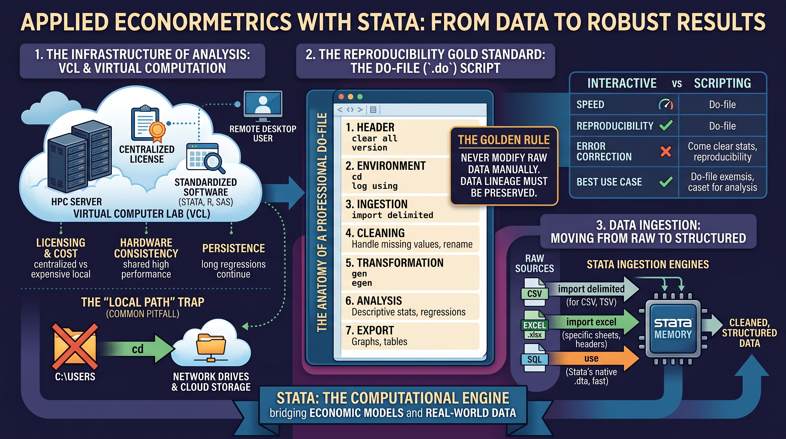
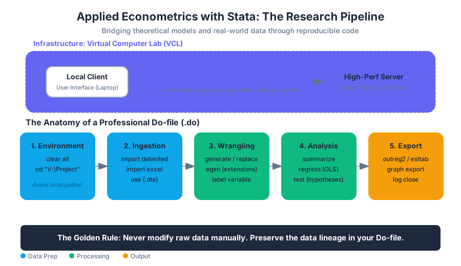
A Virtual Computer Lab (VCL) is a remote-access environment that provides users with a standardized suite of software (like Stata, R, or SAS) without requiring local installation. It operates on a client-server model where the heavy computation occurs on a high-performance server, while the user interacts via a remote desktop protocol.
Why it matters
The VCL solves three critical problems:
- Licensing and Cost: Stata licenses can be prohibitively expensive for individual students; the VCL centralizes this cost.
- Hardware Consistency: It ensures that every student is working with the same processing power and memory, preventing "it works on my machine" errors during large-scale data joins.
- Persistence: Research sessions can often be "disconnected" rather than "logged out," allowing long-running regressions to continue executing even if the user's local laptop loses internet connectivity.
Common Pitfalls: The "Local Path" Trap
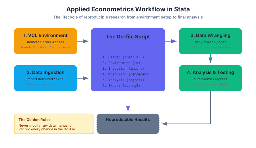
A frequent error in the VCL environment is the mismanagement of file paths. Because the VCL is a remote machine, it has its own file system. Users often try to reference files on their local C:\Users\Documents folder, which the VCL cannot see. Researchers must use the cd (change directory) command to point Stata toward the VCL’s network drives or cloud-mapped storage.
The Gold Standard: Do-files and Reproducibility
In econometrics, the result is only as good as the path taken to reach it. Reproducibility is the requirement that an independent researcher can take your raw data and code and produce the exact same results.
What it is
A Do-file (.do) is a plain-text script containing a sequence of Stata commands. Instead of typing commands one-by-one into the "Command" window (interactive mode), the researcher writes the entire pipeline in the Do-file editor and executes it in one go.
The Anatomy of a Professional Do-file
A robust Do-file follows a specific structural hierarchy:
- Header: Version control, memory clearing (
clear all), and logging (log using). - Environment: Setting the working directory (
cd). - Ingestion: Importing raw data.
- Cleaning: Handling missing values, renaming variables, and labeling.
- Transformation: Creating new variables (
gen,egen). - Analysis: Descriptive statistics and regressions.
- Export: Saving results to tables or graphs.
The Golden Rule of Do-files: Never modify your raw data manually. Every change—from dropping an outlier to renaming a column—must be recorded in the Do-file so the "data lineage" is preserved.
| Feature | Interactive Command Window | Do-file Scripting |
|---|---|---|
| Speed | Fast for quick checks | Slower to set up |
| Reproducibility | Zero; history is lost on exit | High; permanent record |
| Error Correction | Must re-type everything | Edit one line and re-run |
| Complexity | Limited to simple tasks | Handles multi-stage pipelines |
| Best Use Case | Browsing data (br) |
Final analysis and HW submissions |
Data Ingestion: Moving from Raw to Structured
Data rarely arrives in Stata's native .dta format. It usually exists as CSVs, Excel spreadsheets, or SQL exports.
Importing Mechanics
Stata provides several engines for data ingestion. The choice depends on the source format and the presence of metadata (like column headers).
import delimited: The modern standard for CSV and text files. It is highly flexible and automatically detects delimiters (commas, tabs, semicolons).import excel: Specifically designed for.xlsxfiles. It allows the researcher to specify which sheet to load and whether the first row contains variable names.use: Used exclusively for Stata's proprietary.dtafiles. It is the fastest method because the data is already structured for Stata's memory.
Implementation Example: The Ingestion Pipeline
// 1. Low-level implementation of a data setup script
capture log close               // Close any open logs
log using "analysis_log.txt", replace

clear all                       // Clear memory
set more off                    // Prevent "more" prompts

// Set the working directory (VCL specific path example)
cd "V:\Economics\Project1"

// Import raw CSV data
import delimited "raw_census_data.csv", case(lower) clear

// Basic data audit
describe                        // Check variable types
summarize                       // Check for impossible values (e.g., age = -1)
list in 1/10                    // Peek at the first 10 observations
Variable Transformation and Data Wrangling
Once data is loaded, it is rarely ready for regression. Econometricians spend roughly 80% of their time in the Data Wrangling phase—transforming raw inputs into theoretically sound variables.
The generate vs. replace Logic
generate(orgen): Creates a brand new variable in the dataset.replace: Modifies the values of an existing variable.egen(Extensions to Generate): Used for complex transformations like calculating means across groups or creating standardized scores (z-scores).
Dummy Variables (Indicator Variables)
A dummy variable is a binary variable that takes the value 1 if a condition is true and 0 otherwise. These are crucial for modeling qualitative differences (e.g., Gender, Treatment vs. Control, or Regional effects).
Mathematical Derivation of Variable Transformation
In a multiple linear regression, we often transform variables to satisfy the Gauss-Markov assumptions or to model non-linear relationships. For example, the Log-Log model is used to estimate elasticities.
\begin{aligned}
\text{Raw Model:} & \quad Y = \beta_0 X^{\beta_1} e^u \\
\text{Transformation:} & \quad \ln(Y) = \ln(\beta_0) + \beta_1 \ln(X) + u \\
\text{Stata Logic:} & \quad \text{gen ln_y = ln(y)} \\
& \quad \text{gen ln_x = ln(x)} \\
& \quad \text{reg ln_y ln_x}
\end{aligned}
Table: Common Transformation Patterns
| Goal | Stata Command | Economic Interpretation |
|---|---|---|
| Interaction | gen x1_x2 = x1 * x2 |
How the effect of $x_1$ changes with $x_2$ |
| Quadratic | gen x_sq = x^2 |
Modeling U-shaped or Diminishing returns |
| Binary | gen treated = (income > 50000) |
Creating a threshold-based group |
| Group Mean | egen avg_inc = mean(inc), by(state) |
Comparing individuals to their peers |
Exploratory Data Analysis (EDA) with Scatterplots
Before running a regression, one must "look" at the data. Visual inspection can reveal outliers, non-linearity, or heteroskedasticity that summary statistics might hide.
The twoway scatter Command
The scatterplot is the primary tool for visualizing the relationship between two continuous variables. In Stata, the twoway command allows for layering, such as plotting a scatterplot and an OLS regression line (the "best fit" line) simultaneously.
Implementation: Visualizing the Relationship
# Third code block: CLI/Shell-style representation of a Stata batch run
# This demonstrates how a researcher might run a script from the terminal
# to generate a plot without opening the GUI.

stata-mp -b do "visualize_returns_to_schooling.do"

# Inside the .do file:
# twoway (scatter wage educ) (lfit wage educ), ///
#        title("Returns to Education") ///
#        xtitle("Years of Schooling") ytitle("Hourly Wage") ///
#        note("Source: 2023 Labor Survey")
# graph export "output_plot.png", replace
Why Scatterplots Matter
- Outlier Detection: A single data point (e.g., a billionaire in a poverty study) can pull the OLS line away from the true trend.
- Heteroskedasticity: If the "spread" of the dots increases as $X$ increases (a fan shape), the standard errors are likely biased, necessitating the
robustcommand. - Non-linearity: If the dots form a curve, a simple linear model (
reg y x) is misspecified.
Advanced Modeling: IV and Difference-in-Differences
As highlighted in the Homework 5 solutions and final exam preparation, applied econometrics moves beyond simple OLS to address Endogeneity and Causal Inference.
Instrumental Variables (IV)
When an explanatory variable $X$ is correlated with the error term $u$ (due to omitted variable bias or simultaneity), OLS is biased. We use an Instrument (Z) that is correlated with $X$ but uncorrelated with $u$.
Stata Syntax: ivregress 2sls y (x = z) w1 w2, robust
Difference-in-Differences (DID)
DID is used to estimate the causal effect of a policy or treatment by comparing the change in outcomes over time between a treatment group and a control group.
The DID Equation: $$Y_{it} = \beta_0 + \beta_1 \text{Treat}_i + \beta_2 \text{Post}_t + \delta(\text{Treat}_i \times \text{Post}t) + \epsilon{it}$$
In Stata, the coefficient of interest ($\delta$) is the interaction term.
Table: Comparison of Regression Estimators
| Method | Command | Use Case | Key Assumption |
|---|---|---|---|
| OLS | reg y x |
Baseline correlation | $E[u\vert x] = 0$ (Exogeneity) |
| Robust OLS | reg y x, robust |
When variance is not constant | Handles Heteroskedasticity |
| IV (2SLS) | ivregress 2sls ... |
Endogenous regressors | Instrument Validity & Relevance |
| Fixed Effects | xtreg y x, fe |
Panel data (repeated obs) | Time-invariant unobservables |
Preparation for the Final Exam: Logistics and Strategy
Based on the instructor's guidance, the final exam is a high-stakes assessment of both theoretical understanding and practical application.
Exam Parameters
- Duration: 2 hours (Note: Adjusted from 3 hours).
- Materials: 4 double-sided sheets of notes and a calculator.
- Focus Areas: Multiple Linear Regression, Dummy Variables, IV, and DID.
Strategic Advice for Applied Questions
- Show Your Work: Partial credit is awarded for the logic of the derivation, even if the final calculation is off.
- Interpret the Coefficients: Don't just find $\beta_1 = 0.5$. Explain that "a one-unit increase in $X$ is associated with a 0.5 unit increase in $Y$, holding all other factors constant."
- Check for Robustness: If a question mentions "non-constant variance," always specify that you would use the
, robustoption in Stata.
Appendix: Troubleshooting Common Stata Errors
| Error Code | Meaning | Solution |
|---|---|---|
| r(601) | File not found | Check your cd and file spelling. |
| r(111) | Variable not found | You likely forgot to gen it or misspelled it. |
| r(103) | Too many variables | Check your regression syntax; you might have a comma in the wrong place. |
| r(2000) | No observations | Your if condition or missing data handling dropped everyone. |
"The most powerful tool in Stata isn't the
regresscommand; it's thehelpcommand. Typinghelp [command]provides the full documentation, syntax, and examples needed to solve almost any implementation hurdle."
Source Materials
Study Econometric Theory and Empirical Analysis with Stata on Lykke
This course page is free to open: signed out, you can read its first two sections, and signing in, on any plan, opens the rest. The free Lykke Chrome extension syncs your own Canvas courses, so ChatGPT, Claude and Muse can answer from your classes and deadlines. It only reads Canvas.
Add the free extensionSign in to open every sectionAll sections of Econometric Theory and Empirical Analysis with Stata · Browse more course pages