From the free course Econometric Theory and Empirical Analysis with Stata on Lykke
Simple Linear Regression Model
Key concepts: OLS Estimators · Zero Conditional Mean · Unbiasedness · SLR.1-SLR.4 · Sampling Distribution
Covers the mechanics of the two-variable regression model, the OLS estimation method, and the assumptions required for unbiasedness.
Simple Linear Regression Model
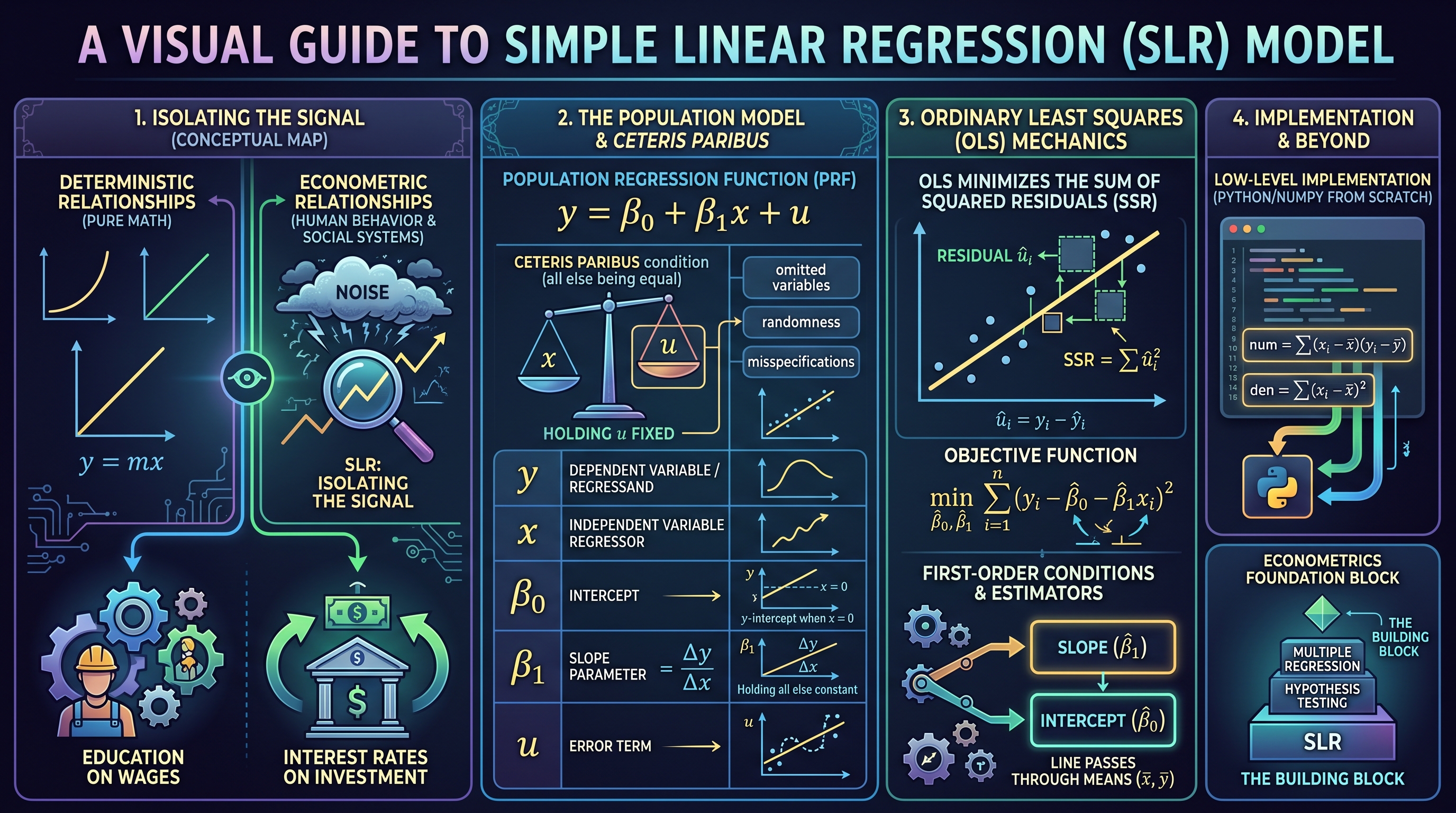
The Simple Linear Regression (SLR) model serves as the foundational building block of econometrics. It provides a formal mathematical framework for estimating the relationship between a dependent variable and a single independent variable. Unlike pure mathematics, where relationships are deterministic, econometrics acknowledges the inherent "noise" in human behavior and social systems. The SLR model attempts to isolate the signal—the systematic relationship between variables—from this noise.
At its core, the SLR model is a tool for empirical analysis, allowing researchers to test economic theories, evaluate policy interventions, and forecast future trends. Whether we are analyzing the impact of education on wages, the effect of interest rates on investment, or the relationship between advertising spend and sales, the SLR model provides the rigorous structure necessary to move from anecdotal observation to statistical inference.
The Population Model and Ceteris Paribus
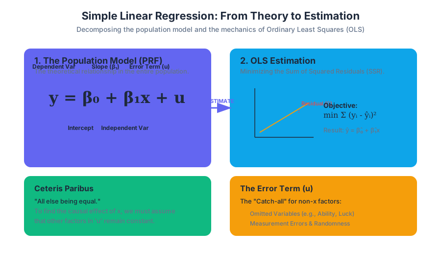
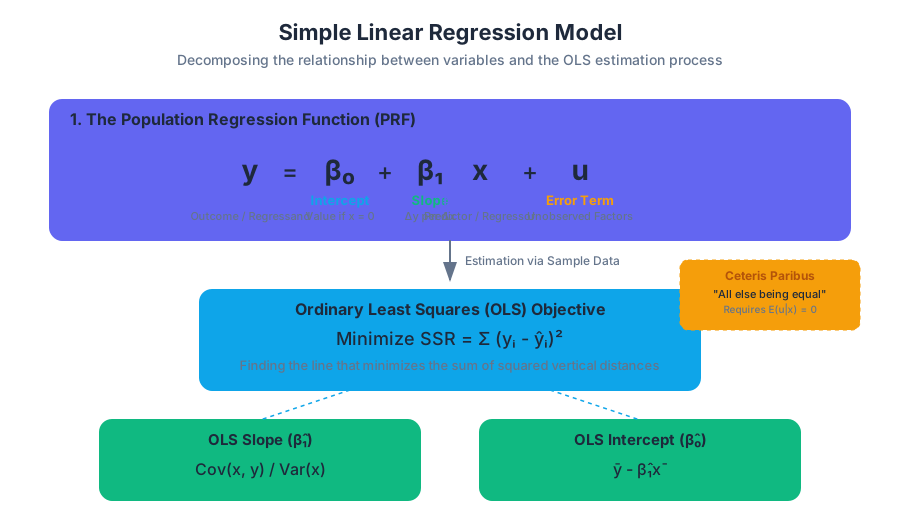
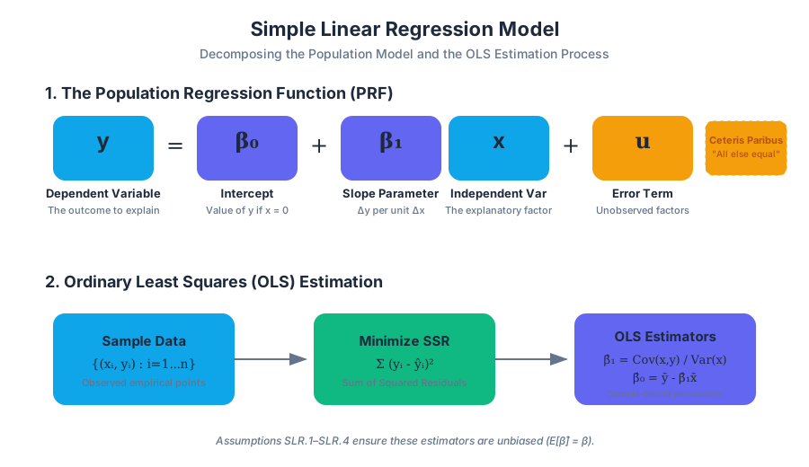
The SLR model describes how a dependent variable $y$ changes as an independent variable $x$ changes in the population. The relationship is expressed by the Population Regression Function (PRF):
$$y = \beta_0 + \beta_1 x + u$$
In this equation, we distinguish between several critical components:
| Component | Term | Definition |
|---|---|---|
| $y$ | Dependent Variable | The variable we are trying to explain (also called the regressand or response variable). |
| $x$ | Independent Variable | The variable used to explain $y$ (also called the regressor, predictor, or explanatory variable). |
| $\beta_0$ | Intercept | The predicted value of $y$ when $x = 0$. |
| $\beta_1$ | Slope Parameter | The change in $y$ for a one-unit change in $x$, holding all other factors constant. |
| $u$ | Error Term | The "disturbance" representing all factors other than $x$ that affect $y$. |
The primary challenge in econometrics is the Ceteris Paribus (all else being equal) condition. Because $u$ contains all other factors affecting $y$, we can only claim that $\beta_1$ represents the causal effect of $x$ on $y$ if we can effectively "hold $u$ fixed." If $x$ is correlated with factors inside $u$, we cannot distinguish the effect of $x$ from the effect of those hidden factors.
Definition: The Error Term ($u$) The error term $u$ is not merely a measurement error. It captures omitted variables, inherent randomness in human behavior, and functional form misspecifications. In a model of
wage = β0 + β1(education) + u, the error term $u$ includes innate ability, work ethic, and family connections.
Ordinary Least Squares (OLS) Mechanics
How do we estimate the unknown parameters $\beta_0$ and $\beta_1$ using a sample of data? The standard method is Ordinary Least Squares (OLS). OLS works by choosing estimates ($\hat{\beta}_0$ and $\hat{\beta}_1$) that minimize the distance between the observed data points and the fitted regression line.
Specifically, OLS minimizes the Sum of Squared Residuals (SSR). For any observation $i$, the residual $\hat{u}_i$ is the difference between the actual value $y_i$ and the predicted value $\hat{y}_i$:
$$\hat{u}_i = y_i - \hat{y}_i = y_i - (\hat{\beta}_0 + \hat{\beta}_1 x_i)$$
The OLS objective function is: $$\min_{\hat{\beta}_0, \hat{\beta}1} \sum{i=1}^{n} (y_i - \hat{\beta}_0 - \hat{\beta}_1 x_i)^2$$
The First-Order Conditions
To find the minimum, we take partial derivatives with respect to $\hat{\beta}_0$ and $\hat{\beta}_1$ and set them to zero. This yields the OLS estimators:
- The Slope ($\hat{\beta}_1$): $\hat{\beta}_1 = \frac{\sum (x_i - \bar{x})(y_i - \bar{y})}{\sum (x_i - \bar{x})^2} = \frac{\text{Cov}(x,y)}{\text{Var}(x)}$
- The Intercept ($\hat{\beta}_0$): $\hat{\beta}_0 = \bar{y} - \hat{\beta}_1 \bar{x}$
These formulas ensure that the regression line passes through the sample means $(\bar{x}, \bar{y})$.
Low-Level Implementation (Python/NumPy)
The following code demonstrates how to implement the OLS closed-form solution from scratch using matrix operations and summation logic.
import numpy as np

def simple_linear_regression(x, y):
    """
    Computes OLS estimators for a simple linear regression.
    Formula: beta_1 = Cov(x,y) / Var(x)
             beta_0 = mean(y) - beta_1 * mean(x)
    """
    n = len(x)
    x_mean = np.mean(x)
    y_mean = np.mean(y)

    # Calculate the numerator (covariance-like) and denominator (variance-like)
    numerator = np.sum((x - x_mean) * (y - y_mean))
    denominator = np.sum((x - x_mean)**2)

    # Slope (beta_1)
    beta_1 = numerator / denominator

    # Intercept (beta_0)
    beta_0 = y_mean - (beta_1 * x_mean)

    # Calculate residuals and R-squared
    y_pred = beta_0 + beta_1 * x
    residuals = y - y_pred
    ssr = np.sum(residuals**2)
    sst = np.sum((y - y_mean)**2)
    r_squared = 1 - (ssr / sst)

    return {
        "intercept": beta_0,
        "slope": beta_1,
        "r_squared": r_squared,
        "residuals": residuals
    }

# Example Usage with synthetic data
x_data = np.array([12, 14, 16, 18, 20]) # Years of Education
y_data = np.array([30, 35, 42, 48, 55]) # Hourly Wage
results = simple_linear_regression(x_data, y_data)

print(f"Model: Wage = {results['intercept']:.2f} + {results['slope']:.2f} * Education")
print(f"R-squared: {results['r_squared']:.4f}")
The Gauss-Markov Assumptions (SLR.1 - SLR.4)
For OLS estimators to be reliable, certain conditions must be met. In the context of "Simple Linear Regression," we focus on the first four Gauss-Markov assumptions, which guarantee that our estimators are unbiased.
SLR.1: Linear in Parameters
The population model must be linear in the parameters $\beta_0$ and $\beta_1$. Note that the variables $x$ and $y$ can be non-linear (e.g., $y = \beta_0 + \beta_1 x^2 + u$), but the coefficients must appear in a linear additive form.
SLR.2: Random Sampling
We have a random sample of $n$ observations ${(x_i, y_i) : i=1, ..., n}$ following the population model. This ensures that the sample is representative of the population we wish to study.
SLR.3: Sample Variation in $x$
The values of $x_i$ in the sample are not all the same. If $x$ is constant, we cannot observe how $y$ changes in response to $x$, and the denominator in the $\hat{\beta}_1$ formula becomes zero, making the estimator undefined.
SLR.4: Zero Conditional Mean
This is the most critical and frequently violated assumption. It states that the error term $u$ has an expected value of zero given any value of $x$: $$E[u|x] = 0$$
If this holds, $x$ is said to be exogenous. If $x$ is correlated with $u$ (i.e., $E[u|x] \neq 0$), then $x$ is endogenous, and the OLS estimator will be biased.
| Assumption | Formal Statement | Violation Consequence | Real-world Example of Violation |
|---|---|---|---|
| SLR.1 | $y = \beta_0 + \beta_1 x + u$ | Model Misspecification | Relationship is exponential, not linear. |
| SLR.2 | ${(x_i, y_i)}$ is IID | Selection Bias | Surveying only wealthy people for a wage study. |
| SLR.3 | $\text{Var}(x) > 0$ | Undefined Estimator | Testing the effect of "Year" using data from only 2023. |
| SLR.4 | $E[u|x] = 0$ | Bias (Inaccuracy) | Omitted variable: "Ability" correlated with "Education". |
Deep Dive: The Zero Conditional Mean Assumption
The assumption $E[u|x] = 0$ implies two things:
- $E[u] = 0$: On average, the factors in the error term cancel out. This is usually trivial because we can always adjust the intercept $\beta_0$ to make this true.
- $\text{Cov}(x, u) = 0$: The unobserved factors are not correlated with the explanatory variable.
Consider the model: $\text{Wage} = \beta_0 + \beta_1 \text{Educ} + u$. If $u$ contains "Ability," and higher-ability individuals tend to get more education, then $\text{Cov}(\text{Educ}, \text{Ability}) > 0$. In this case, OLS will attribute the effect of ability to education, resulting in an "Upward Bias." The estimated $\hat{\beta}_1$ will be larger than the true causal effect $\beta_1$.
Mathematical Derivation of the Slope Estimator
The following block represents the algebraic derivation of the OLS slope estimator, showing how the "Zero Conditional Mean" assumption allows us to identify the population parameter.
1. Start with the definition of covariance:
   Cov(x, y) = Cov(x, beta_0 + beta_1 * x + u)

2. Use covariance properties (linearity):
   Cov(x, y) = Cov(x, beta_0) + Cov(x, beta_1 * x) + Cov(x, u)

3. Simplify:
   - Cov(x, beta_0) = 0 (covariance with a constant is zero)
   - Cov(x, beta_1 * x) = beta_1 * Var(x)
   - Cov(x, u) = 0 (By Assumption SLR.4)

4. Resulting Equation:
   Cov(x, y) = beta_1 * Var(x)

5. Solve for beta_1:
   beta_1 = Cov(x, y) / Var(x)

6. Sample Analog (OLS):
   hat_beta_1 = [Sum(x_i - mean_x)(y_i - mean_y)] / [Sum(x_i - mean_x)^2]
Unbiasedness and the Sampling Distribution
It is vital to distinguish between the Estimator (the rule/formula) and the Estimate (the specific number calculated from a specific sample).
Because the sample is random (SLR.2), $\hat{\beta}_1$ is a random variable. If we took 1,000 different samples from the same population, we would get 1,000 different values for $\hat{\beta}_1$.
Theorem: Unbiasedness of OLS Under assumptions SLR.1 through SLR.4, the OLS estimators are unbiased. That is: $E[\hat{\beta}_0] = \beta_0$ and $E[\hat{\beta}_1] = \beta_1$
Unbiasedness does not mean $\hat{\beta}_1$ will equal $\beta_1$ in any single sample. It means that if we could repeat the sampling process infinitely many times, the average of all those estimates would exactly equal the true population parameter.
Visualizing the Sampling Distribution
The variance of the sampling distribution tells us how "spread out" our estimates are. A smaller variance means our estimator is more precise. The variance of $\hat{\beta}_1$ (under the additional assumption of homoskedasticity) is: $$\text{Var}(\hat{\beta}_1) = \frac{\sigma^2}{\sum (x_i - \bar{x})^2}$$ Where $\sigma^2$ is the variance of the error term $u$.
Goodness of Fit: R-Squared ($R^2$)
Once we have estimated the model, we want to know how well the independent variable $x$ explains the variation in $y$. We decompose the Total Sum of Squares (SST) into two parts:
- SST (Total Sum of Squares): $\sum (y_i - \bar{y})^2$ — Total variation in $y$.
- SSE (Explained Sum of Squares): $\sum (\hat{y}_i - \bar{y})^2$ — Variation explained by the model.
- SSR (Residual Sum of Squares): $\sum \hat{u}_i^2$ — Variation left unexplained.
The relationship is: $SST = SSE + SSR$.
The Coefficient of Determination ($R^2$) is defined as: $$R^2 = \frac{SSE}{SST} = 1 - \frac{SSR}{SST}$$
$R^2$ ranges from 0 to 1. An $R^2$ of 0.30 means that 30% of the variation in $y$ is explained by $x$. In social sciences, $R^2$ is often low (e.g., 0.1 to 0.2) because human behavior is influenced by countless factors outside the model.
| Metric | Formula | Interpretation |
|---|---|---|
| SST | $\sum (y_i - \bar{y})^2$ | The "total uncertainty" in the dependent variable. |
| SSR | $\sum (y_i - \hat{y}_i)^2$ | The "failure" of the model; what we couldn't explain. |
| SSE | $\sum (\hat{y}_i - \bar{y})^2$ | The "success" of the model; the movement in $y$ tracked by $x$. |
| $R^2$ | $SSE / SST$ | Percentage of variance explained (0 to 100%). |
Practical Implementation in Stata
In professional econometrics, software like Stata is the industry standard for performing these calculations. Stata handles the matrix algebra internally and provides robust diagnostic output.
// 1. Load a dataset (e.g., the 'attend' dataset from Wooldridge)
use http://www.stata.com/data/jwooldridge/econtf/attend.dta, clear

// 2. Summarize variables to check SLR.3 (variation in x)
summarize atndrte priGPA

// 3. Visualize the relationship (Scatterplot with regression line)
twoway (scatter atndrte priGPA) (lfit atndrte priGPA)

// 4. Run the Simple Linear Regression
// Syntax: regress [dependent] [independent]
regress atndrte priGPA

/*
Output Interpretation:
- '_cons' is the intercept (beta_0)
- 'priGPA' coefficient is the slope (beta_1)
- 'R-squared' is the goodness of fit
- 'Prob > F' tests if the model is statistically significant
*/

// 5. Predict residuals to check for patterns
predict u_hat, residual
scatter u_hat priGPA, yline(0)
Common Pitfalls and Misconceptions
1. Correlation is Not Causation
Just because $\hat{\beta}_1$ is statistically significant does not mean $x$ causes $y$. If SLR.4 is violated (e.g., omitted variable bias), the coefficient represents both the effect of $x$ and the effect of the correlated unobservables.
2. The "Intercept" Fallacy
Often, the intercept $\beta_0$ has no meaningful economic interpretation. For example, in a regression of weight on height, the intercept represents the weight of a person with zero height. While mathematically necessary to anchor the line, it is often outside the range of observed data.
3. Low $R^2$ Does Not Mean a "Bad" Model
A low $R^2$ is common in cross-sectional data. A researcher might have a very precise and unbiased estimate of a small effect. The goal of econometrics is often to estimate $\beta_1$ accurately, not necessarily to predict $y$ perfectly.
4. Non-Linearity
If the true relationship is a curve (e.g., diminishing marginal returns), a straight line will provide a poor fit and potentially biased estimates of the local effect. This is why visual inspection of data (scatterplots) is a mandatory first step.
Summary of the SLR Workflow
- Specify the Theory: Define $y$ and $x$ and the expected sign of $\beta_1$.
- Collect Data: Ensure the sample is random (SLR.2).
- Inspect Data: Check for variation in $x$ (SLR.3) and potential non-linearity.
- Estimate OLS: Calculate $\hat{\beta}_0$ and $\hat{\beta}_1$.
- Evaluate Assumptions: Critically assess if $E[u|x]=0$ (SLR.4).
- Interpret Results: Use the slope to describe the ceteris paribus effect and $R^2$ to describe the fit.
Source Materials
Study Econometric Theory and Empirical Analysis with Stata on Lykke
This course page is free to open: signed out, you can read its first two sections, and signing in, on any plan, opens the rest. The free Lykke Chrome extension syncs your own Canvas courses, so ChatGPT, Claude and Muse can answer from your classes and deadlines. It only reads Canvas.
Add the free extensionSign in to open every sectionAll sections of Econometric Theory and Empirical Analysis with Stata · Browse more course pages