From the free course Econometric Theory and Empirical Analysis with Stata on Lykke
Multiple Regression: Estimation and Inference
Key concepts: Partial Effects · Omitted Variable Bias · Gauss-Markov Theorem (BLUE) · t-tests · F-tests
Extends the regression framework to multiple independent variables, focusing on partial effects, the Gauss-Markov Theorem, and hypothesis testing.
Multiple Regression: Estimation and Inference
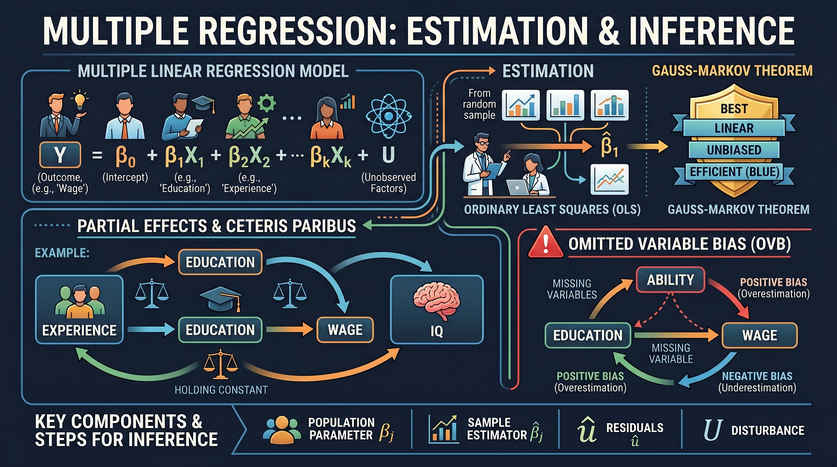
Multiple Linear Regression (MLR) is the cornerstone of empirical economic analysis. While Simple Linear Regression (SLR) provides a foundation, it rarely suffices in the real world where outcomes are driven by a complex web of interrelated factors. The power of MLR lies in its ability to isolate the effect of a single variable while "holding constant" other confounding factors—a concept known as ceteris paribus.
In this deep dive, we move beyond basic correlation to explore how MLR allows for rigorous estimation of partial effects, the dangers of omitting crucial variables, and the statistical framework required to make valid inferences about population parameters.
The Multiple Linear Regression Model
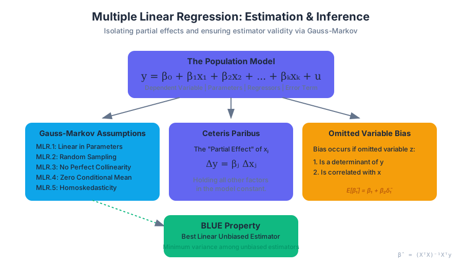
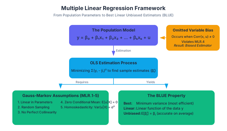
The population model for multiple linear regression with $k$ independent variables is expressed as:
$$y = \beta_0 + \beta_1 x_1 + \beta_2 x_2 + \dots + \beta_k x_k + u$$
Where:
- $y$ is the dependent variable (the outcome we wish to explain).
- $x_1, x_2, \dots, x_k$ are the independent variables (regressors or predictors).
- $\beta_0$ is the intercept (the value of $y$ if all $x$ are zero).
- $\beta_1, \dots, \beta_k$ are the slope parameters (measuring the partial effect of each $x$).
- $u$ is the error term (representing unobserved factors affecting $y$).
| Component | Description | Role in Inference |
|---|---|---|
| $\beta_j$ | Population Parameter | The "true" relationship we seek to estimate. |
| $\hat{\beta}_j$ | OLS Estimator | The sample-based estimate of the population parameter. |
| $u$ | Disturbance/Error | The source of uncertainty; must satisfy Gauss-Markov assumptions. |
| $\hat{u}$ | Residual | The difference between observed $y$ and predicted $\hat{y}$. |
Partial Effects: The "Ceteris Paribus" Interpretation
The primary motivation for using MLR over SLR is the partial effect interpretation. In a simple regression, the coefficient on $x$ often captures the effects of other variables correlated with $x$. In MLR, the coefficient $\beta_j$ measures the change in $y$ for a one-unit change in $x_j$, holding all other independent variables in the model constant.
Mathematical Intuition
If we have the model $y = \beta_0 + \beta_1 x_1 + \beta_2 x_2 + u$, the partial effect of $x_1$ is: $$\frac{\Delta y}{\Delta x_1} = \beta_1$$ This derivative holds $x_2$ and $u$ fixed. This allows us to mimic an experimental setting using non-experimental (observational) data. For example, in a model of wages, we can estimate the effect of education while holding years of experience and IQ constant.
Omitted Variable Bias (OVB)
One of the most significant challenges in econometrics is Omitted Variable Bias. This occurs when we exclude a variable from our regression that is both:
- A determinant of $y$ (i.e., it belongs in the error term $u$).
- Correlated with one or more of the included independent variables.
The Mechanics of Bias
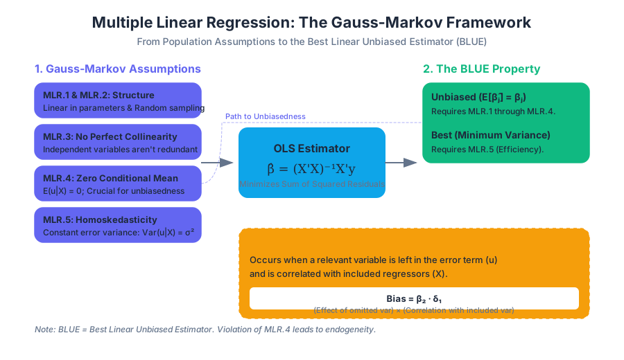
Suppose the "true" population model is: $$y = \beta_0 + \beta_1 x_1 + \beta_2 x_2 + u$$ If we mistakenly estimate a model that excludes $x_2$: $$\tilde{y} = \tilde{\beta}_0 + \tilde{\beta}_1 x_1 + \tilde{u}$$ The estimator $\tilde{\beta}_1$ will generally be biased. The relationship between the biased estimator and the true parameter is: $$E[\tilde{\beta}_1] = \beta_1 + \beta_2 \tilde{\delta}_1$$ where $\tilde{\delta}_1$ is the slope coefficient from a regression of the omitted variable ($x_2$) on the included variable ($x_1$).
Direction of Bias
The direction of the bias depends on the signs of $\beta_2$ (the effect of the omitted variable on $y$) and $Corr(x_1, x_2)$.
| $Corr(x_1, x_2) > 0$ | $Corr(x_1, x_2) < 0$ | |
|---|---|---|
| $\beta_2 > 0$ | Positive Bias (Overestimation) | Negative Bias (Underestimation) |
| $\beta_2 < 0$ | Negative Bias (Underestimation) | Positive Bias (Overestimation) |
Professor's Note: If the omitted variable is uncorrelated with the included regressor ($\tilde{\delta}_1 = 0$), the OLS estimator remains unbiased, though it may be less efficient.
The Gauss-Markov Theorem: Why OLS?
Ordinary Least Squares (OLS) is the most widely used estimation method because, under specific conditions, it possesses ideal statistical properties. These conditions are known as the Gauss-Markov Assumptions.
The MLR Assumptions (MLR.1 - MLR.5)
- MLR.1: Linear in Parameters: The model in the population can be written as $y = \beta_0 + \beta_1 x_1 + \dots + \beta_k x_k + u$.
- MLR.2: Random Sampling: We have a random sample of $n$ observations following the population model.
- MLR.3: No Perfect Collinearity: In the sample, none of the independent variables is constant, and there are no exact linear relationships among the independent variables.
- MLR.4: Zero Conditional Mean: The error $u$ has an expected value of zero given any values of the independent variables: $E[u | x_1, \dots, x_k] = 0$.
- MLR.5: Homoskedasticity: The error $u$ has the same variance given any values of the explanatory variables: $Var(u | x_1, \dots, x_k) = \sigma^2$.
The BLUE Property
Theorem: Under assumptions MLR.1 through MLR.5, the OLS estimators $\hat{\beta}_0, \hat{\beta}_1, \dots, \hat{\beta}_k$ are the Best Linear Unbiased Estimators (BLUE).
- Best: Minimum variance (most efficient) among all linear unbiased estimators.
- Linear: The estimator is a linear function of the data ($y$).
- Unbiased: On average, the estimator equals the true population parameter ($E[\hat{\beta}_j] = \beta_j$).
Implementation: OLS via Matrix Algebra
In a professional or computational context, MLR is solved using matrix algebra. This is more efficient than solving $k+1$ simultaneous equations manually.
import numpy as np

def manual_ols(X, y):
    """
    Implements OLS estimation using the Normal Equation:
    beta_hat = (X^T * X)^-1 * X^T * y
    """
    # Add a column of ones to X for the intercept beta_0
    n_obs = X.shape[0]
    X_with_intercept = np.hstack([np.ones((n_obs, 1)), X])

    # Calculate (X^T * X)^-1
    xtx = np.dot(X_with_intercept.T, X_with_intercept)
    xtx_inv = np.linalg.inv(xtx)

    # Calculate X^T * y
    xty = np.dot(X_with_intercept.T, y)

    # Final beta coefficients
    beta_hat = np.dot(xtx_inv, xty)

    # Residuals and Variance Estimation
    residuals = y - np.dot(X_with_intercept, beta_hat)
    dof = n_obs - X_with_intercept.shape[1]
    sigma_squared = np.sum(residuals**2) / dof

    # Variance-Covariance Matrix of coefficients
    var_beta = sigma_squared * xtx_inv
    std_errors = np.sqrt(np.diagonal(var_beta))

    return beta_hat, std_errors

# Example Usage
X_data = np.array([[15, 2], [18, 3], [20, 5], [22, 5], [25, 7]]) # e.g., Education, Experience
y_data = np.array([30, 35, 42, 48, 55]) # e.g., Wage
betas, se = manual_ols(X_data, y_data)
print(f"Coefficients: {betas}")
print(f"Std Errors: {se}")
Statistical Inference: The t-test
Once we have our estimates $\hat{\beta}_j$, we need to determine if they are statistically significant—that is, whether we can confidently say they are different from zero in the population.
The t-statistic
To test the null hypothesis $H_0: \beta_j = 0$ against the alternative $H_1: \beta_j \neq 0$, we calculate the t-statistic: $$t_{\hat{\beta}_j} = \frac{\hat{\beta}_j}{se(\hat{\beta}_j)}$$ Where $se(\hat{\beta}_j)$ is the standard error of the estimator. Under the Classical Linear Model (CLM) assumptions (which add normality of errors to MLR.1-MLR.5), this statistic follows a $t$-distribution with $n - k - 1$ degrees of freedom.
Decision Rules
- p-value approach: If the p-value is less than the significance level $\alpha$ (usually 0.05), reject $H_0$.
- Critical value approach: If $|t| > t_{critical}$, reject $H_0$.
\text{Standard Error of } \hat{\beta}_j: \\
se(\hat{\beta}_j) = \sqrt{\frac{\hat{\sigma}^2}{SST_j(1 - R_j^2)}} \\
\\
\text{where } SST_j \text{ is total variation in } x_j, \\
\text{and } R_j^2 \text{ is the R-squared from regressing } x_j \text{ on all other } x\text{'s.}
Joint Significance: The F-test
Sometimes we want to test multiple hypotheses simultaneously. For example, we might ask: "Do experience and tenure jointly affect wages, even if neither is significant individually?"
Restricted vs. Unrestricted Models
To perform an F-test, we compare two models:
- Unrestricted Model (UR): The full model with all variables.
- Restricted Model (R): The model where the null hypothesis is imposed (e.g., the coefficients of the variables being tested are set to zero).
The F-statistic is calculated as: $$F = \frac{(SSR_r - SSR_{ur}) / q}{SSR_{ur} / (n - k - 1)}$$ Where:
- $SSR_r$ is the Sum of Squared Residuals from the restricted model.
- $SSR_{ur}$ is the Sum of Squared Residuals from the unrestricted model.
- $q$ is the number of restrictions (number of variables being tested).
- $n - k - 1$ is the degrees of freedom of the unrestricted model.
| Feature | t-test | F-test |
|---|---|---|
| Scope | Single coefficient | Multiple coefficients (joint) |
| Hypothesis | $\beta_j = 0$ | $\beta_1 = \beta_2 = \dots = \beta_q = 0$ |
| Distribution | $t_{n-k-1}$ | $F_{q, n-k-1}$ |
| Direction | One-tailed or Two-tailed | Always One-tailed (right-tail) |
Functional Forms: Non-linear Relationships
MLR is "linear in parameters," but the variables themselves can be non-linear. This allows for immense flexibility in modeling.
Logarithmic Transformations
Log transformations are used to model percentage changes (elasticities).
- Log-Log Model: $\log(y) = \beta_0 + \beta_1 \log(x) + u$. $\beta_1$ is the elasticity of $y$ with respect to $x$.
- Log-Linear Model: $\log(y) = \beta_0 + \beta_1 x + u$. $100 \cdot \beta_1$ is the percentage change in $y$ for a one-unit change in $x$.
- Linear-Log Model: $y = \beta_0 + \beta_1 \log(x) + u$. $\beta_1 / 100$ is the change in $y$ for a 1% change in $x$.
Quadratic Forms
To capture "diminishing marginal returns," we use squared terms: $$y = \beta_0 + \beta_1 x + \beta_2 x^2 + u$$ The marginal effect of $x$ is no longer constant: $\frac{\Delta y}{\Delta x} = \beta_1 + 2\beta_2 x$. If $\beta_1 > 0$ and $\beta_2 < 0$, the relationship follows an inverted U-shape.
Real-World Application: Stata Workflow
In practice, researchers use specialized software like Stata to handle these calculations and perform diagnostic tests.
// Load dataset (e.g., wage data)
use "http://www.stata-press.com/data/r15/nlsw88.dta", clear

// 1. Estimate Multiple Regression
// wage: dependent variable
// educ, exper, tenure: independent variables
regress wage educ exper tenure

// 2. Test for Omitted Variable Bias (Ramsey RESET test)
ovtest

// 3. Perform a t-test on a specific coefficient (automatic in 'regress' output)
// But we can also test specific values:
test educ = 1.5

// 4. Perform an F-test for joint significance of exper and tenure
test exper tenure

// 5. Generate a non-linear model (Quadratic experience)
gen exper2 = exper^2
regress wage educ exper exper2 tenure

// 6. Visualizing the partial effect of education
avplot educ
Common Pitfalls and Misconceptions
- Mistaking $R^2$ for Model Quality: A high $R^2$ does not mean the model is "good" or that the estimates are unbiased. It simply means the $x$ variables explain a lot of the variation in $y$. In social sciences, low $R^2$ values (0.1 - 0.3) are very common.
- The "Everything but the Kitchen Sink" Approach: Adding too many variables to avoid OVB can lead to Multicollinearity, which inflates standard errors and makes estimates unstable.
- Correlation vs. Causation: Even with many controls, MLR only establishes causality if the Zero Conditional Mean assumption (MLR.4) holds. If an unobserved factor (like "innate ability") is correlated with both education and wages, the coefficient on education is still biased.
- Interpreting Logs: Forgetting to multiply by 100 when interpreting log-linear models is a frequent student error.
Summary of Inference Logic
The journey from data to insight in MLR follows a strict logical pipeline:
- Specify the model based on economic theory.
- Collect data and ensure it meets the random sampling assumption.
- Estimate coefficients using OLS.
- Check Gauss-Markov assumptions (especially linearity and homoskedasticity).
- Evaluate statistical significance using t-tests for individual variables and F-tests for groups.
- Interpret the magnitude of the coefficients in the context of the units (or logs) used.
Source Materials
Study Econometric Theory and Empirical Analysis with Stata on Lykke
This course page is free to open: signed out, you can read its first two sections, and signing in, on any plan, opens the rest. The free Lykke Chrome extension syncs your own Canvas courses, so ChatGPT, Claude and Muse can answer from your classes and deadlines. It only reads Canvas.
Add the free extensionSign in to open every sectionAll sections of Econometric Theory and Empirical Analysis with Stata · Browse more course pages