From the free course Econometric Theory and Empirical Analysis with Stata on Lykke
Introduction and Statistical Foundations
Key concepts: Ceteris Paribus · Causality vs. Correlation · Empirical Analysis Steps · Counterfactuals
Establishes the definition of econometrics and the fundamental distinction between causality and correlation, alongside a review of essential statistical concepts.
Introduction and Statistical Foundations
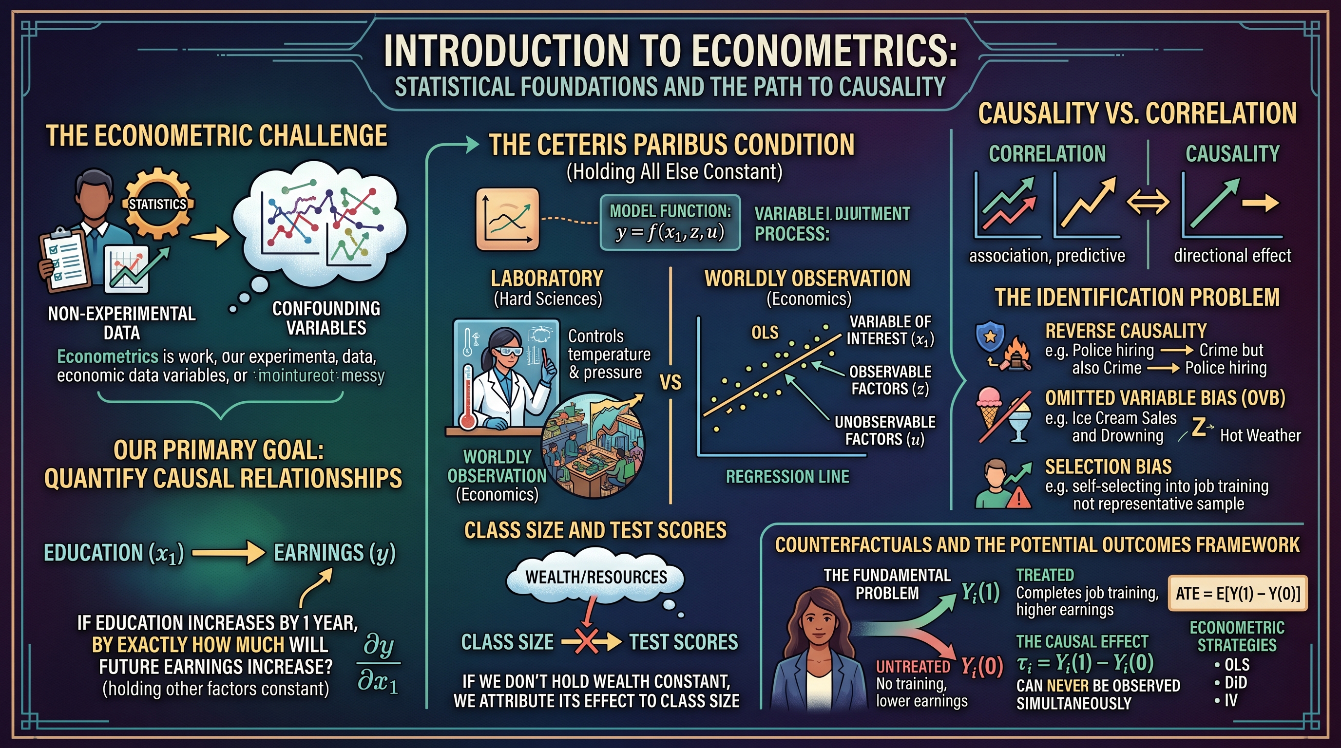
Econometrics is the rigorous application of mathematical and statistical methods to the analysis of economic data. While it shares a lineage with mathematical statistics, econometrics is a distinct discipline because it focuses on the unique challenges of non-experimental data. In the hard sciences, researchers can often control the environment; in economics, we observe the world as it is, fraught with confounding variables and complex interdependencies.
The primary goal of econometrics is not merely to find patterns, but to quantify causal relationships. We do not just ask if education and earnings move together; we ask: "If we increase a person's education by one year, by exactly how much will their future earnings increase, holding all other factors constant?"
The Ceteris Paribus Condition
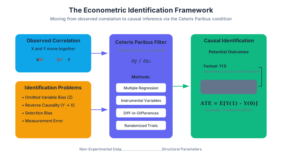
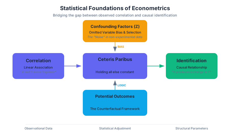
The cornerstone of economic theory and econometric estimation is the Ceteris Paribus condition—a Latin phrase meaning "holding all else constant." In a laboratory, a chemist can hold temperature and pressure constant while varying a catalyst. In economics, we must use statistical techniques to mimic this control.
The Mathematical Representation
In a functional relationship $y = f(x_1, x_2, ..., x_n)$, the effect of $x_1$ on $y$ is defined by the partial derivative: $$\frac{\partial y}{\partial x_1}$$ This derivative represents the change in $y$ for a marginal change in $x_1$, assuming $x_2$ through $x_n$ remain unchanged. In econometrics, our models explicitly partition the world into the variable of interest ($x$), other observable factors ($z$), and unobservable factors ($u$).
Why Ceteris Paribus is Difficult
In observational data, variables are rarely independent. If we want to measure the effect of "Class Size" on "Student Test Scores," we face the problem that wealthier school districts often have both smaller classes and more resources at home. If we simply compare small classes to large classes without "holding constant" family income, we attribute the effect of wealth to class size.
| Data Type | Control Mechanism | Primary Challenge |
|---|---|---|
| Experimental | Random Assignment | Cost, Ethics, External Validity |
| Observational | Statistical Adjustment (Regression) | Omitted Variable Bias, Endogeneity |
| Quasi-Experimental | Natural Shocks (DiD, IV) | Finding a "clean" natural experiment |
Causality vs. Correlation
A common mantra in statistics is that "correlation does not imply causation." Econometrics takes this a step further by defining exactly why they differ and how to close the gap.
- Correlation: A measure of the linear association between two variables. If $X$ and $Y$ are correlated, knowing $X$ helps us predict $Y$.
- Causality: A directional relationship where a change in $X$ produces a change in $Y$.
The Identification Problem
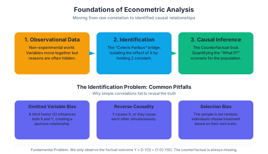
The central struggle in econometrics is Identification. We say a causal effect is "identified" if we can isolate it from the noise of other correlations. Consider the relationship between police presence and crime rates. A simple correlation might show that cities with more police have higher crime. A naive observer might conclude police cause crime. In reality, the causality is reversed: high-crime cities hire more police. This is known as Simultaneous Equation Bias.
Common Pitfalls in Causal Logic
- Reverse Causality: $Y$ causes $X$ instead of $X$ causing $Y$.
- Omitted Variable Bias (OVB): A third variable $Z$ causes both $X$ and $Y$, creating a "spurious" correlation.
- Selection Bias: The sample is not representative, or individuals "self-select" into the treatment group based on characteristics that also affect the outcome.
Counterfactuals and the Potential Outcomes Framework
To understand causality, we must think in terms of Counterfactuals. A counterfactual asks: "What would have happened to this specific individual if they had received a different treatment?"
The Potential Outcomes Notation
Let $Y_i(1)$ be the outcome for individual $i$ if they receive the treatment (e.g., a job training program), and $Y_i(0)$ be the outcome if they do not. The Causal Effect for individual $i$ is: $$\tau_i = Y_i(1) - Y_i(0)$$
The Fundamental Problem of Causal Inference is that we can never observe both $Y_i(1)$ and $Y_i(0)$ for the same person at the same time. We only observe the "factual" outcome: $$Y_i = D_i Y_i(1) + (1 - D_i) Y_i(0)$$ where $D_i$ is a binary indicator (1 if treated, 0 if not).
Average Treatment Effect (ATE)
Since we cannot calculate $\tau_i$ for individuals, we aim for the population average: $$ATE = E[Y(1) - Y(0)]$$ Econometric methods like OLS, Difference-in-Differences, and Instrumental Variables are all different strategies to estimate this ATE by constructing a valid proxy for the missing counterfactual.
import numpy as np
import pandas as pd

# Low-level implementation: Simulating Potential Outcomes and Selection Bias
def simulate_causal_data(n=1000):
    # 1. Generate unobserved ability (the 'u' in our model)
    ability = np.random.normal(10, 2, n)

    # 2. Treatment assignment (Education) is NOT random
    # People with higher ability are more likely to get more education
    education = 0.5 * ability + np.random.normal(8, 1, n)

    # 3. Define Potential Outcomes
    # Wage if Education = x: Wage = 5 + 2*Education + 1*Ability + noise
    # Note: Ability affects both Education and Wage (Omitted Variable Bias)
    noise = np.random.normal(0, 1, n)
    wage = 5 + 2 * education + 1 * ability + noise

    df = pd.DataFrame({
        'wage': wage,
        'education': education,
        'ability': ability # In the real world, we wouldn't see this!
    })

    # Simple Correlation (Biased)
    naive_beta = df['wage'].cov(df['education']) / df['education'].var()

    # True Causal Effect (from our formula above) is 2.0
    print(f"Naive OLS Estimate: {naive_beta:.4f}")
    print(f"True Causal Effect: 2.0000")

    return df

simulate_causal_data()
The Empirical Analysis Process
A structured econometric study follows a specific pipeline. It is not enough to simply "run a regression"; one must ground the analysis in theory and data integrity.
Steps in Empirical Analysis
- Question Formulation: Define a narrow, testable hypothesis (e.g., "Does reducing class size by 10% increase test scores?").
- Economic Model: Write down a theoretical framework. This might be a utility maximization problem or a simple behavioral assumption.
- Econometric Model: Convert the economic model into a functional form that can be estimated.
- Example: $Score = \beta_0 + \beta_1 ClassSize + \beta_2 Income + u$
- Data Collection: Identify the population, sampling scheme, and unit of observation.
- Estimation: Use software (like Stata or R) to calculate the parameters ($\hat{\beta}$).
- Hypothesis Testing: Determine if the results are statistically significant or likely due to chance.
| Step | Goal | Common Tool |
|---|---|---|
| Specification | Define the relationship | Linear Regression Equation |
| Identification | Ensure $\beta$ is causal | Instrumental Variables, Fixed Effects |
| Inference | Test significance | t-stats, p-values, F-tests |
| Diagnostics | Check assumptions | Residual plots, Breusch-Pagan test |
Simple Linear Regression (SLR) Foundations
The Simple Linear Regression model is the workhorse of econometrics. It relates a dependent variable $y$ to a single independent variable $x$ via the equation: $$y = \beta_0 + \beta_1 x + u$$
The Gauss-Markov Assumptions (SLR.1 - SLR.4)
To ensure that our OLS estimators ($\hat{\beta}_0, \hat{\beta}_1$) are unbiased (meaning that on average, they hit the true population parameter), four assumptions must hold:
- SLR.1: Linear in Parameters: The population model must be linear in $\beta_0$ and $\beta_1$. (Note: $x$ can be non-linear, like $x^2$).
- SLR.2: Random Sampling: The data represents a random draw from the population.
- SLR.3: Sample Variation in X: The values of $x$ in our sample cannot all be the same. We need variation to see how $y$ changes.
- SLR.4: Zero Conditional Mean: This is the "Golden Rule." It states that the error term $u$ has an expected value of zero regardless of the value of $x$: $$E[u|x] = 0$$
The Zero Conditional Mean Assumption is the mathematical embodiment of ceteris paribus. If $E[u|x] \neq 0$, it means that some factors hidden in $u$ are correlated with $x$. This violates the "holding all else constant" requirement, leading to biased estimates.
Deriving the OLS Estimator
The goal of Ordinary Least Squares (OLS) is to minimize the Sum of Squared Residuals (SSR).
% Mathematical Derivation of Beta_1
To minimize SSR = \sum (y_i - \hat{\beta}_0 - \hat{\beta}_1 x_i)^2:

1. Take the partial derivative with respect to \hat{\beta}_1:
   \frac{\partial SSR}{\partial \hat{\beta}_1} = -2 \sum x_i (y_i - \hat{\beta}_0 - \hat{\beta}_1 x_i) = 0

2. Solving the system of first-order conditions yields:
   \hat{\beta}_1 = \frac{\sum (x_i - \bar{x})(y_i - \bar{y})}{\sum (x_i - \bar{x})^2}

3. Which is equivalent to:
   \hat{\beta}_1 = \frac{Cov(x, y)}{Var(x)}
Advanced Topic: Multiple Regression and Partialling Out
In the real world, SLR is rarely sufficient because of Omitted Variable Bias. Multiple Linear Regression (MLR) allows us to include multiple control variables: $$y = \beta_0 + \beta_1 x_1 + \beta_2 x_2 + ... + \beta_k x_k + u$$
The "Partialling Out" Interpretation
In a multiple regression, $\beta_1$ has a very specific meaning. It is the effect of $x_1$ on $y$ after the effects of $x_2, ..., x_k$ have been "partialled out" or removed from both $x_1$ and $y$. This is the statistical realization of the ceteris paribus thought experiment.
| Concept | SLR | MLR |
|---|---|---|
| Model | $y = \beta_0 + \beta_1 x + u$ | $y = \beta_0 + \beta_1 x_1 + \beta_2 x_2 + u$ |
| Interpretation | Total association | Partial effect (ceteris paribus) |
| Error Term | Contains all other factors | Contains only factors not in model |
| Bias Risk | High (Omitted variables) | Lower (if controls are good) |
Practical Implementation in Stata
Stata is the industry standard for econometric research due to its robust handling of complex survey data and built-in commands for causal inference.
Standard Workflow
A typical session involves cleaning data, generating new variables (transformations), and running regressions with robust standard errors to account for heteroskedasticity.
// 1. Setup environment
clear all
set more off
capture log close

// 2. Load dataset (Example: Wage and Education)
use "http://www.stata-press.com/data/r15/wage2.dta", clear

// 3. Descriptive Statistics
summarize wage educ exper tenure

// 4. Visualizing the relationship
twoway (scatter wage educ) (lfit wage educ), title("Wage vs Education")

// 5. Simple Linear Regression
regress wage educ

// 6. Multiple Regression with Ceteris Paribus controls
// We add 'exper' (experience) and 'tenure' to hold them constant
regress wage educ exper tenure, robust

// 7. Testing a hypothesis (e.g., does educ coefficient = 100?)
test educ = 100
Common Pitfalls in Empirical Foundations
Even with sophisticated software, researchers often fall into traps that invalidate their causal claims.
1. The Dummy Variable Trap
When using categorical data (e.g., "Gender" or "Region"), one must always omit one category (the "base group"). If you include a dummy for "Male" and a dummy for "Female" along with an intercept, the model will suffer from perfect multicollinearity because $Male + Female = 1$ (the constant).
2. Over-controlling (Bad Controls)
While adding controls is generally good for ceteris paribus, adding "bad controls" can introduce bias. A bad control is a variable that is itself an outcome of the variable of interest. For example, if studying the effect of education on wages, controlling for "Job Title" is problematic because education helps determine your job title.
3. Misinterpreting R-Squared
A high $R^2$ (the fraction of variance explained by the model) does not mean the model is "good" or "causal." In time-series data, two unrelated variables that both trend upward over time will have an $R^2$ near 1.0, despite having zero causal connection. This is known as Spurious Regression.
Summary of Statistical Properties
To wrap up the foundations, we must distinguish between the Estimator (the rule/formula) and the Estimate (the number produced by a specific sample).
- Unbiasedness: $E[\hat{\beta}] = \beta$. On average, the estimator is correct.
- Efficiency: Among all unbiased estimators, the one with the smallest variance is the most efficient.
- Consistency: As the sample size $n$ approaches infinity, the estimate $\hat{\beta}$ collapses to the true population value $\beta$.
The Gauss-Markov Theorem: Under assumptions SLR.1 through SLR.5 (adding Homoskedasticity), the OLS estimator is the BLUE: Best Linear Unbiased Estimator.
Source Materials
Study Econometric Theory and Empirical Analysis with Stata on Lykke
This course page is free to open: signed out, you can read its first two sections, and signing in, on any plan, opens the rest. The free Lykke Chrome extension syncs your own Canvas courses, so ChatGPT, Claude and Muse can answer from your classes and deadlines. It only reads Canvas.
Add the free extensionSign in to open every sectionAll sections of Econometric Theory and Empirical Analysis with Stata · Browse more course pages