From the free course Econometric Theory and Empirical Analysis with Stata on Lykke
Qualitative Data and Advanced Causal Inference
Key concepts: Dummy Variable Trap · Linear Probability Model (LPM) · Instrumental Variables (IV) · Difference-in-Differences (DiD)
Introduces dummy variables for categorical data and advanced methods for identifying causal effects in the presence of endogeneity.
Qualitative Data and Advanced Causal Inference
In the rigorous pursuit of economic truth, we often find that the most compelling questions involve variables that cannot be measured on a continuous scale—gender, race, employment status, or the presence of a specific policy. Furthermore, the "gold standard" of experimental design is rarely available to social scientists. We are frequently left with observational data where the variables of interest are endogenous, meaning they are correlated with the very error terms we hope to minimize.
This section explores the transition from simple linear models to sophisticated causal frameworks. We begin by formalizing the treatment of qualitative information through dummy variables, navigate the pitfalls of the Linear Probability Model, and conclude with the pillars of modern causal inference: Instrumental Variables (IV) and Difference-in-Differences (DiD).
Qualitative Information and Dummy Variables
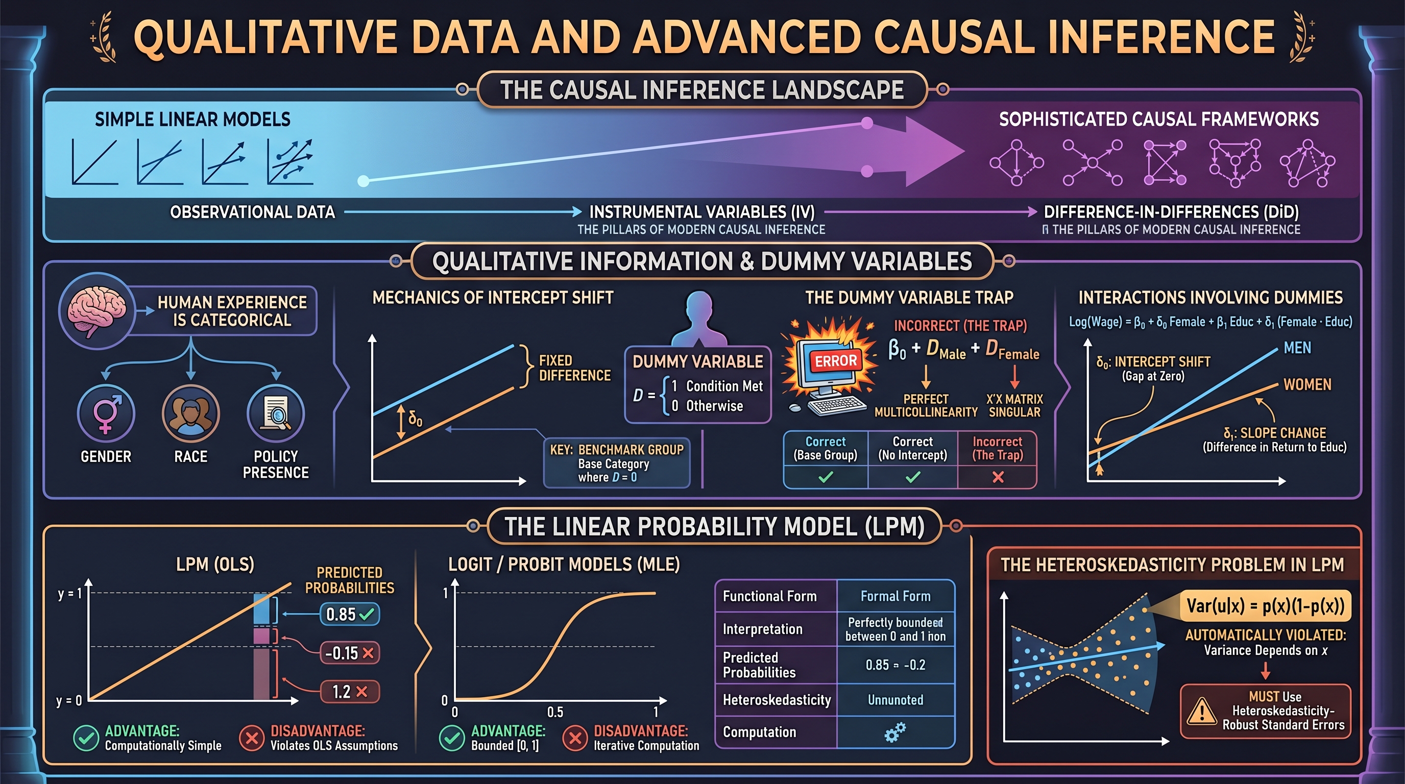
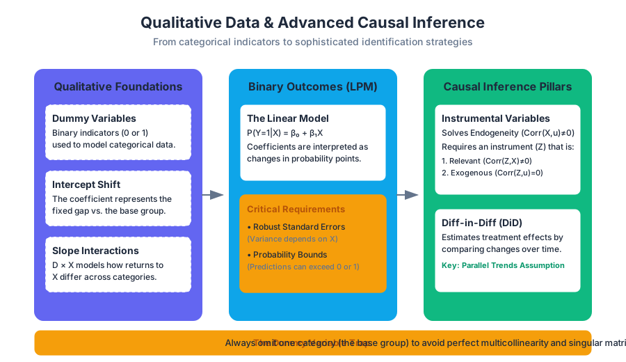
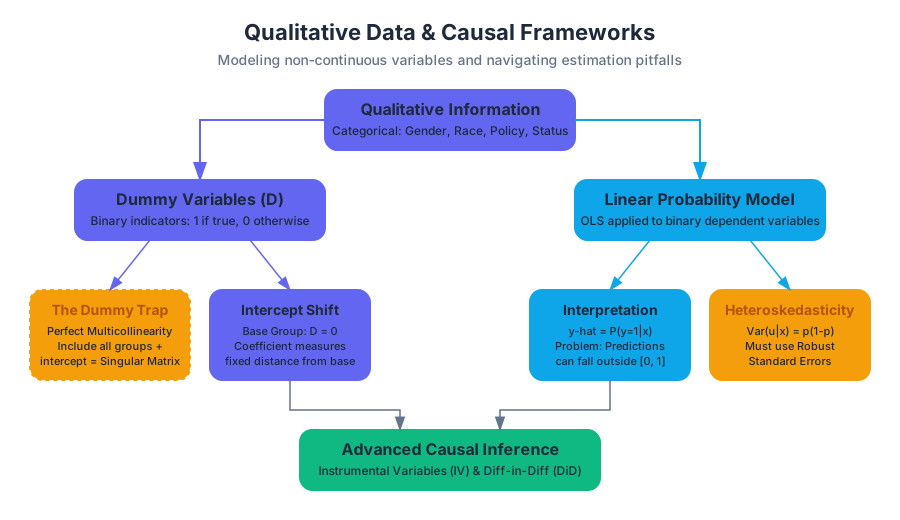
In standard regression, we assume variables like income or distance are continuous. However, much of human experience is categorical. To incorporate this into a linear framework, we use Dummy Variables (also known as binary or indicator variables).
A dummy variable $D$ is defined as: $$D = \begin{cases} 1 & \text{if the condition is met} \ 0 & \text{otherwise} \end{cases}$$
The Mechanics of the Intercept Shift
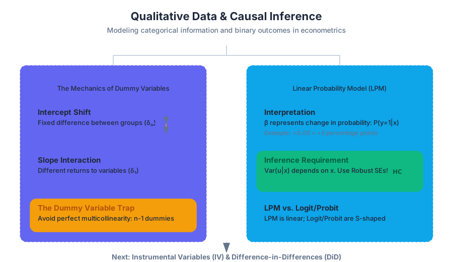
When we include a dummy variable in a regression, such as $Wage = \beta_0 + \delta_0 Female + \beta_1 Exper + u$, the coefficient $\delta_0$ represents a fixed difference in the intercept between the two groups.
Definition: The Benchmark Group In any model containing dummy variables, the group for which the dummy is 0 is referred to as the base group, benchmark group, or omitted category. All dummy coefficients are interpreted as the expected difference relative to this base group, ceteris paribus.
The Dummy Variable Trap
A common error for novice econometricians is attempting to include a dummy variable for every possible category in a set while also retaining the intercept. This leads to perfect multicollinearity.
If you have two categories (e.g., Male and Female) and you include $D_{male}$, $D_{female}$, and an intercept $\beta_0$, the model cannot be estimated. This is because $D_{male} + D_{female} = 1$ for every observation, which is exactly equal to the constant associated with the intercept. The matrix $X'X$ becomes singular and non-invertible.
| Strategy | Specification | Result |
|---|---|---|
| Correct (Base Group) | $Y = \beta_0 + \beta_1 D_1 + u$ | $\beta_0$ is the mean of group 0; $\beta_1$ is the difference. |
| Correct (No Intercept) | $Y = \alpha_1 D_0 + \alpha_2 D_1 + u$ | $\alpha_1$ and $\alpha_2$ are the absolute means of each group. |
| Incorrect (The Trap) | $Y = \beta_0 + \beta_1 D_0 + \beta_2 D_1 + u$ | Failure: Perfect multicollinearity; Stata/R will drop one variable. |
Interactions Involving Dummies
We can also model differences in slopes by interacting a dummy with a continuous variable. $$Log(Wage) = \beta_0 + \delta_0 Female + \beta_1 Educ + \delta_1 (Female \cdot Educ) + u$$ In this case:
- $\delta_0$ is the "gender gap" for someone with zero education.
- $\delta_1$ is the difference in the return to education between men and women.
The Linear Probability Model (LPM)
When the dependent variable ($y$) is binary, we enter the realm of discrete choice modeling. The simplest approach is the Linear Probability Model (LPM), where we use OLS to estimate a binary outcome.
Interpretation
In an LPM, the predicted value $\hat{y}$ is interpreted as the probability that $y=1$ given the values of $x$. $$P(y=1|x) = \beta_0 + \beta_1 x_1 + \dots + \beta_k x_k$$ The coefficient $\beta_j$ represents the change in the probability of the event occurring for a one-unit increase in $x_j$, holding other factors constant.
Advantages and Disadvantages
While computationally simple and highly interpretable, the LPM violates several standard OLS assumptions.
| Feature | Linear Probability Model (LPM) | Logit / Probit Models |
|---|---|---|
| Functional Form | Linear: $x\beta$ | Non-linear: $\Lambda(x\beta)$ or $\Phi(x\beta)$ |
| Interpretation | Marginal effect is constant ($\beta$) | Marginal effect depends on $x$ |
| Predicted Probabilities | Can be $<0$ or $>1$ (nonsensical) | Strictly bounded between 0 and 1 |
| Heteroskedasticity | Always present by construction | Handled via Maximum Likelihood |
| Computation | OLS (Fast, closed-form) | Iterative (Slower) |
The Heteroskedasticity Problem in LPM
In a binary model, the variance of the error term $u$ is $Var(u|x) = p(x)(1-p(x))$, where $p(x)$ is the probability of success. Since this variance depends on $x$, the Gauss-Markov assumption of homoskedasticity is automatically violated.
Critical Insight: To obtain valid inference (t-stats and p-values) in an LPM, you must use heteroskedasticity-robust standard errors.
# Low-level implementation of LPM with Robust Standard Errors
import numpy as np
import pandas as pd

def estimate_lpm_robust(X, y):
    """
    Estimates a Linear Probability Model with White's Robust Standard Errors.
    X: Design matrix (including intercept)
    y: Binary dependent variable
    """
    # 1. OLS Coefficients: beta = (X'X)^-1 X'y
    xtx_inv = np.linalg.inv(X.T @ X)
    beta = xtx_inv @ X.T @ y

    # 2. Residuals
    y_hat = X @ beta
    residuals = y - y_hat

    # 3. Robust Covariance Matrix (HC1)
    # Sigma = (X'X)^-1 * (sum of e_i^2 * x_i * x_i') * (X'X)^-1
    n, k = X.shape
    meat = np.zeros((k, k))
    for i in range(n):
        row = X[i, :].reshape(1, -1)
        meat += (residuals[i]**2) * (row.T @ row)

    # Degrees of freedom adjustment (n / (n-k))
    df_adj = n / (n - k)
    vcov = df_adj * (xtx_inv @ meat @ xtx_inv)

    se = np.sqrt(np.diag(vcov))
    return beta, se

# Example usage with synthetic data
# X = [1, educ, exper], y = employed (0 or 1)
Instrumental Variables (IV) and 2SLS
One of the most profound challenges in econometrics is Endogeneity. This occurs when $Cov(x, u) \neq 0$, violating the Zero Conditional Mean assumption (MLR.4). This usually stems from:
- Omitted Variable Bias (e.g., "Ability" affecting both education and wages).
- Measurement Error in the independent variable.
- Simultaneity (e.g., Supply and Demand).
The IV Solution
To solve this, we find an Instrumental Variable ($z$) that satisfies two conditions:
- Instrument Relevance: $Cov(z, x) \neq 0$. The instrument must be correlated with the endogenous regressor.
- Exclusion Restriction (Instrument Exogeneity): $Cov(z, u) = 0$. The instrument must have no direct effect on $y$ and must not be correlated with other unobserved factors.
Two-Stage Least Squares (2SLS)
The standard method for implementing IV is 2SLS.
\text{Step 1: The First Stage}
\\ \text{Regress the endogenous variable } x \text{ on the instrument } z \text{ and all other exogenous variables } w.
\\ x = \pi_0 + \pi_1 z + \pi_2 w + v
\\ \text{Obtain the predicted values: } \hat{x}

\\ \text{Step 2: The Second Stage}
\\ \text{Regress the dependent variable } y \text{ on the predicted values } \hat{x} \text{ and exogenous variables } w.
\\ y = \beta_0 + \beta_1 \hat{x} + \beta_2 w + u
The intuition is that $\hat{x}$ contains only the "clean" variation in $x$ (the part triggered by $z$), which is uncorrelated with $u$.
Derivation of the IV Estimator
In a simple model $y = \beta_0 + \beta_1 x + u$ with instrument $z$: $$Cov(z, y) = Cov(z, \beta_0 + \beta_1 x + u)$$ $$Cov(z, y) = \beta_1 Cov(z, x) + Cov(z, u)$$ Since $Cov(z, u) = 0$ by assumption: $$\beta_{1, IV} = \frac{Cov(z, y)}{Cov(z, x)}$$
| Metric | OLS Estimator | IV Estimator |
|---|---|---|
| Consistency | Inconsistent if $Cov(x, u) \neq 0$ | Consistent if $z$ is valid |
| Efficiency | More efficient (smaller variance) | Less efficient (larger variance) |
| Bias | Biased in small samples | Biased in small samples (but consistent) |
| Requirement | $E[u | x] = 0$ |
Common Pitfalls: Weak Instruments
If $Cov(z, x)$ is very small, the instrument is "weak." A weak instrument leads to large standard errors and can actually amplify the bias of OLS if the exclusion restriction is even slightly violated. A common rule of thumb is that the F-statistic from the first-stage regression should be greater than 10.
Difference-in-Differences (DiD)
Difference-in-Differences is a quasi-experimental technique used to estimate the causal effect of a specific intervention or policy change. It mimics a randomized control trial by comparing the changes in outcomes over time between a "treatment" group and a "control" group.
The Logic of DiD
Imagine a state increases its minimum wage (Treatment), while a neighboring state does not (Control). We cannot simply compare the treatment group before and after, because other things might have changed over time (e.g., a national recession). We cannot simply compare the two states after the change, because they might have been different to begin with.
DiD calculates the "difference of the differences":
- Difference 1: Change in the treatment group $(Y_{T, post} - Y_{T, pre})$.
- Difference 2: Change in the control group $(Y_{C, post} - Y_{C, pre})$.
- DiD Estimate: $(Y_{T, post} - Y_{T, pre}) - (Y_{C, post} - Y_{C, pre})$.
The Regression Specification
The DiD estimate is easily obtained using an interaction term: $$Y_{it} = \beta_0 + \beta_1 Treat_i + \beta_2 Post_t + \delta (Treat_i \cdot Post_t) + \epsilon_{it}$$
- $Treat_i$: Dummy for being in the treatment group.
- $Post_t$: Dummy for the period after the intervention.
- $\delta$: The DiD coefficient, representing the causal effect of the treatment.
| Group | Pre-Treatment | Post-Treatment | Difference |
|---|---|---|---|
| Control | $\beta_0$ | $\beta_0 + \beta_2$ | $\beta_2$ |
| Treatment | $\beta_0 + \beta_1$ | $\beta_0 + \beta_1 + \beta_2 + \delta$ | $\beta_2 + \delta$ |
| Diff-in-Diff | $\delta$ |
The Parallel Trends Assumption
The validity of DiD rests entirely on the Parallel Trends Assumption: in the absence of the treatment, the difference between the treatment and control groups would have remained constant over time.
Warning: If the treatment group was already trending upward faster than the control group before the policy change, the DiD estimate will be biased upward, falsely attributing the pre-existing trend to the policy.
// Real-world usage in Stata: Card & Krueger (1994) style
// y = employment, state = (1 for NJ, 0 for PA), time = (1 for post-wage hike)

// 1. Basic DiD using interaction syntax
reg employment i.state##i.time, vce(robust)

// 2. The coefficient on the interaction (1.state#1.time) is the DiD effect

// 3. Testing for Parallel Trends (Placebo Test)
// Use data from periods BEFORE the actual treatment
reg employment i.state##i.pre_period_dummy if time == 0, vce(robust)
// If the interaction is significant here, parallel trends is violated.
Summary of Advanced Causal Methods
Choosing the right tool depends on the nature of your data and the source of endogeneity.
| Method | Best Used When... | Key Requirement |
|---|---|---|
| LPM | $Y$ is binary and interpretability is key. | Robust standard errors. |
| IV / 2SLS | $X$ is endogenous (e.g., choice-based). | A valid, strong instrument ($z$). |
| DiD | There is a clear "event" or policy change. | Parallel trends assumption. |
| Fixed Effects | You have panel data (repeated observations). | Endogeneity is constant over time. |
Extended Study: The Wald Estimator
For a binary instrument and binary treatment, the IV estimator simplifies to the Wald Estimator: $$\beta_{Wald} = \frac{E[y|z=1] - E[y|z=0]}{E[x|z=1] - E[x|z=0]}$$ This is essentially the ratio of the "Intent-to-Treat" (ITT) effect to the "compliance rate." It serves as a foundational bridge between the experimental literature and structural econometrics. When you hear a researcher discuss "Local Average Treatment Effects" (LATE), they are referring to the effect of the treatment specifically on the "compliers"—those whose behavior was actually changed by the instrument.
Source Materials
Study Econometric Theory and Empirical Analysis with Stata on Lykke
This course page is free to open: signed out, you can read its first two sections, and signing in, on any plan, opens the rest. The free Lykke Chrome extension syncs your own Canvas courses, so ChatGPT, Claude and Muse can answer from your classes and deadlines. It only reads Canvas.
Add the free extensionSign in to open every sectionAll sections of Econometric Theory and Empirical Analysis with Stata · Browse more course pages