From the free course Data Structures and Algorithmic Analysis on Lykke
Sorting Methodologies
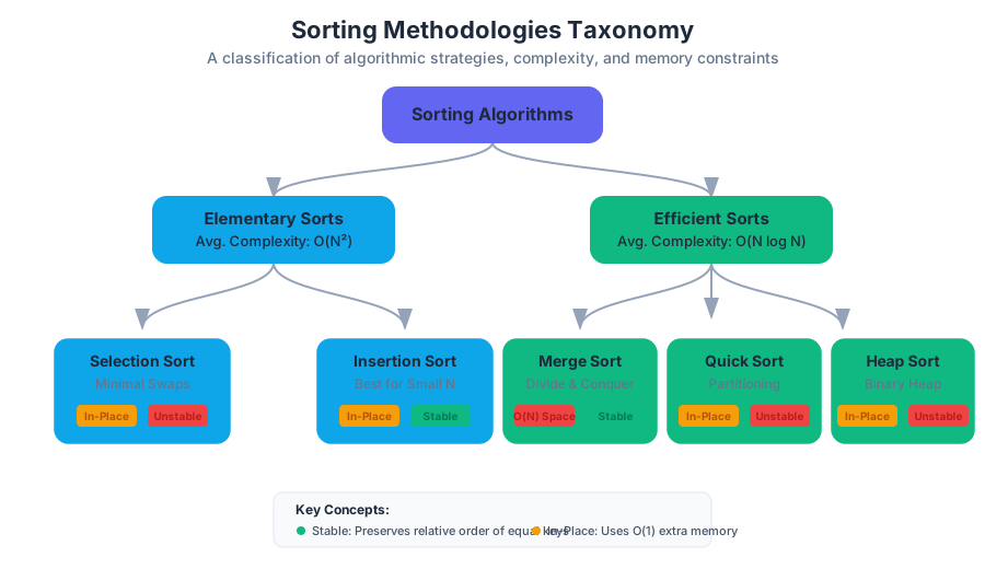
Key concepts: Elementary Sorts (Selection, Insertion) · Merge Sort · Quick Sort · Heap Sort · Stability and In-place Sorting
A deep dive into various sorting algorithms, from elementary methods to efficient divide-and-conquer strategies.
Sorting Methodologies
Sorting is perhaps the most fundamental problem in computational theory. At its surface, it is the process of rearranging a sequence of objects in a specific order (typically numerical or lexicographical). However, beneath this simple definition lies a vast landscape of algorithmic strategies, memory management trade-offs, and mathematical proofs. In a production environment, the "best" sorting algorithm is rarely a single choice but rather a decision based on data distribution, hardware constraints, and stability requirements.
Core Definitions and Taxonomy
Before dissecting specific methodologies, we must establish the metrics by which we judge a sorting algorithm. We do not merely look at "speed"; we look at how that speed scales and how the algorithm interacts with the system's memory.
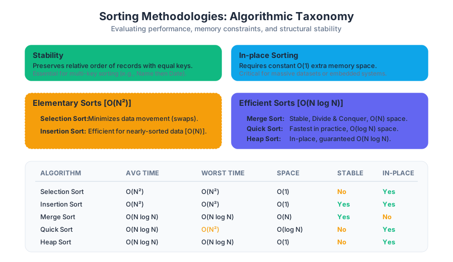
Definition: Stability A sorting algorithm is stable if it preserves the relative order of records with equal keys. If two items $A$ and $B$ have the same key and $A$ appears before $B$ in the original list, a stable sort guarantees $A$ will still appear before $B$ in the sorted list. This is critical when sorting by multiple criteria (e.g., sorting by "First Name" and then "Last Name").
Definition: In-place Sorting An algorithm is in-place if it requires only a constant amount $O(1)$ of extra memory space beyond the original array. This is vital in embedded systems or when handling massive datasets that barely fit into RAM.
Summary of Algorithmic Characteristics
| Algorithm | Best Case | Average Case | Worst Case | Space Complexity | Stable? | In-place? |
|---|---|---|---|---|---|---|
| Selection Sort | $O(N^2)$ | $O(N^2)$ | $O(N^2)$ | $O(1)$ | No | Yes |
| Insertion Sort | $O(N)$ | $O(N^2)$ | $O(N^2)$ | $O(1)$ | Yes | Yes |
| Merge Sort | $O(N \log N)$ | $O(N \log N)$ | $O(N \log N)$ | $O(N)$ | Yes | No |
| Quick Sort | $O(N \log N)$ | $O(N \log N)$ | $O(N^2)$ | $O(\log N)$ | No | Yes |
| Heap Sort | $O(N \log N)$ | $O(N \log N)$ | $O(N \log N)$ | $O(1)$ | No | Yes |
Elementary Sorts
Elementary sorts are characterized by their $O(N^2)$ average-case complexity. While they are inefficient for large $N$, they possess small constant factors and are often used as sub-routines in more complex algorithms.
Selection Sort
Selection Sort is the most intuitive sorting method. It works by dividing the input into a "sorted" sub-list and an "unsorted" sub-list. It repeatedly finds the minimum element from the unsorted sub-list and swaps it with the leftmost unsorted element.
Mechanics:
- Maintain a pointer $i$ starting at 0.
- Scan the array from $i$ to $N-1$ to find the index
minof the smallest element. - Swap
a[i]anda[min]. - Increment $i$ and repeat until the array is exhausted.
Mathematical Analysis: The number of compares in Selection Sort is independent of the initial order of the data. For an array of size $N$, it always performs: $$(N-1) + (N-2) + \dots + 1 + 0 = \frac{N(N-1)}{2} \approx \frac{N^2}{2} \text{ compares.}$$ It performs exactly $N$ swaps. This makes Selection Sort useful when the cost of moving items is very high relative to the cost of comparing them.
Insertion Sort
Insertion Sort functions similarly to how one might sort a hand of playing cards. It processes elements one by one, inserting each into its proper place among the elements already processed.
Mechanics:
- Start with the second element (index 1).
- Compare it with the element to its left. If it is smaller, "slide" the larger elements to the right until the correct hole is found.
- Insert the element.
The Inversion Metric: Insertion Sort's performance is tied to the number of inversions in the array. An inversion is a pair of keys $(a[i], a[j])$ such that $i < j$ but $a[i] > a[j]$.
- If an array is nearly sorted (the number of inversions is $O(N)$), Insertion Sort runs in $O(N)$ time.
- This makes it the algorithm of choice for small arrays ($N < 15$) or for cleaning up data that is already mostly in order.
public class ElementarySorts {
    public static void selectionSort(Comparable[] a) {
        int N = a.length;
        for (int i = 0; i < N; i++) {
            int min = i;
            for (int j = i + 1; j < N; j++) {
                if (less(a[j], a[min])) min = j;
            }
            exch(a, i, min);
        }
    }

    public static void insertionSort(Comparable[] a) {
        int N = a.length;
        for (int i = 1; i < N; i++) {
            for (int j = i; j > 0 && less(a[j], a[j-1]); j--) {
                exch(a, j, j-1);
            }
        }
    }

    private static boolean less(Comparable v, Comparable w) {
        return v.compareTo(w) < 0;
    }

    private static void exch(Object[] a, int i, int j) {
        Object tmp = a[i];
        a[i] = a[j];
        a[j] = tmp;
    }
}
Merge Sort: The Divide and Conquer Paradigm
Merge Sort is a recursive algorithm that achieves the theoretical lower bound for comparison-based sorting: $O(N \log N)$. It is based on the principle that merging two sorted arrays is much easier than sorting a single unsorted one.
Mechanics of the Merge
The heart of the algorithm is the merge operation. Given two sorted halves of an array, we use an auxiliary array to reconstruct the full sorted sequence. We maintain three pointers: one for the left half, one for the right half, and one for the destination in the auxiliary array.
Top-Down vs. Bottom-Up
- Top-Down Merge Sort: This is the standard recursive implementation. It divides the array into halves, calls itself on those halves, and then merges.
- Bottom-Up Merge Sort: This is a non-recursive version. It starts by merging adjacent pairs of elements (size 1), then merges the resulting sorted blocks of size 2, then 4, and so on. This is often preferred in environments where recursion depth is a concern.
Mathematical Proof of Complexity: Let $T(N)$ be the number of compares to sort $N$ elements. The recurrence relation is: $$T(N) = 2T(N/2) + N$$ Using the Master Theorem, where $a=2, b=2, f(n)=n$: Since $n^{\log_b a} = n^{\log_2 2} = n^1$, and $f(n) = \Theta(n)$, we fall into Case 2. Therefore, $T(N) = \Theta(N \log N)$.
Common Pitfalls:
- Memory Overhead: Unlike the elementary sorts, Merge Sort is not in-place. It requires an auxiliary array of size $N$. In memory-constrained environments, this can be a deal-breaker.
- Recursive Depth: For very large $N$, the stack depth could theoretically lead to a
StackOverflowError, though this is rare given the $\log N$ growth.
Quick Sort: The Partitioning Paradigm
Quick Sort is widely considered the most efficient general-purpose sorting algorithm. While it has a worst-case complexity of $O(N^2)$, its average-case performance is $O(1.39 N \log N)$ with very small constant factors.
The Partitioning Step
Quick Sort works by choosing a pivot element and rearranging the array so that:
- The pivot is in its final sorted position.
- All elements to the left of the pivot are less than or equal to it.
- All elements to the right of the pivot are greater than or equal to it.
Mechanics (Hoare Partitioning):
- Pick
a[lo]as the pivot. - Scan
ifrom left to right as long asa[i] < pivot. - Scan
jfrom right to left as long asa[j] > pivot. - Swap
a[i]anda[j]. - Repeat until
iandjcross. - Swap the pivot with
a[j].
The Importance of Randomization
Quick Sort's worst case occurs when the pivot is consistently the smallest or largest element (e.g., sorting an already sorted array). To prevent this, we must shuffle the array before sorting. This guarantees that the $O(N^2)$ case is mathematically improbable (less likely than the computer being struck by a meteor).
Variations: 3-Way Partitioning (Dijkstra's Solution)
When an array contains many duplicate keys, standard Quick Sort still performs $O(N \log N)$ or even $O(N^2)$ work. 3-way partitioning (the Dutch National Flag problem) divides the array into three sections: elements less than the pivot, elements equal to the pivot, and elements greater than the pivot.
public class QuickSort {
    public static void sort(Comparable[] a) {
        StdRandom.shuffle(a); // Crucial for performance guarantee
        sort(a, 0, a.length - 1);
    }

    private static void sort(Comparable[] a, int lo, int hi) {
        if (hi <= lo) return;
        int j = partition(a, lo, hi);
        sort(a, lo, j - 1);
        sort(a, j + 1, hi);
    }

    private static int partition(Comparable[] a, int lo, int hi) {
        int i = lo, j = hi + 1;
        Comparable v = a[lo];
        while (true) {
            while (less(a[++i], v)) if (i == hi) break;
            while (less(v, a[--j])) if (j == lo) break;
            if (i >= j) break;
            exch(a, i, j);
        }
        exch(a, lo, j);
        return j;
    }
}
Heap Sort: Priority Queue Sorting
Heap Sort utilizes a Binary Heap data structure to manage elements. It is essentially a "Selection Sort" but using a sophisticated data structure to find the maximum element in $O(\log N)$ time rather than $O(N)$.
The Two Phases
- Heap Construction: We transform the raw array into a max-heap. This is done in $O(N)$ time using the "bottom-up" heapify method (sinking elements from the middle of the array to the start).
- Sortdown: We repeatedly remove the maximum element (the root of the heap), swap it with the last element of the unsorted portion, and "sink" the new root to restore the heap property.
Advantages:
- Guaranteed $O(N \log N)$: Unlike Quick Sort, there is no "worst-case" $N^2$.
- In-place: Unlike Merge Sort, it uses $O(1)$ extra space.
Disadvantages:
- Cache Locality: Heap Sort jumps around in memory (from index $i$ to $2i$ and $2i+1$). This leads to many cache misses, making it slower in practice than Quick Sort or Merge Sort on modern hardware.
- Not Stable: The swapping process destroys the relative order of equal keys.
| Strategy | Pivot/Structure | Key Advantage | Key Disadvantage |
|---|---|---|---|
| Standard Quick | First element (after shuffle) | Fastest average time | Worst case $O(N^2)$ |
| 3-Way Quick | Pivot with equal-key handling | Efficient for duplicates | Slightly more complex code |
| Heap Sort | Max-Heap structure | Guaranteed $O(N \log N)$ | Poor cache performance |
Stability and In-place Sorting: The Engineering Trade-off
In professional software engineering, the choice of sorting algorithm is often dictated by the nature of the data and the system architecture.
When to use what?
- Java
Arrays.sort(): Uses a variation of TimSort (a hybrid of Merge Sort and Insertion Sort) for Object arrays because stability is usually expected for objects. It uses Dual-Pivot Quick Sort for primitives because stability isn't required and speed is paramount. - Embedded Systems: Heap Sort is often preferred because it provides a hard guarantee on $O(N \log N)$ time and $O(1)$ space, ensuring the system never runs out of memory or hangs on a "bad" dataset.
- Large Scale Data Processing: Merge Sort is the basis for external sorting (sorting data that doesn't fit in RAM) because it accesses data sequentially, which is ideal for disk I/O or tape drives.
Comparison of Stability and Space
| Algorithm | Stable? | In-place? | Notes |
|---|---|---|---|
| Selection | No | Yes | Minimizes swaps. |
| Insertion | Yes | Yes | Best for nearly sorted data. |
| Merge | Yes | No | Guaranteed $N \log N$, high memory. |
| Quick | No | Yes | Fastest in practice, cache-friendly. |
| Heap | No | Yes | Guaranteed $N \log N$, cache-hostile. |
Common Pitfalls and Edge Cases
- The "Sorted Array" Trap: Applying Quick Sort to an already sorted array without shuffling or using a median-of-three pivot selection results in $O(N^2)$ performance.
- Duplicate Keys: Standard Quick Sort can become $O(N^2)$ if all keys are equal. 3-way partitioning is the standard fix.
- Stability Misconception: Many believe that any algorithm can be made stable easily. While true (by adding the original index to the key), it increases space complexity to $O(N)$.
- Comparator Violations: In languages like Java or C++, if your
compareToorcomparefunction does not obey the transitive property (if $a < b$ and $b < c$, then $a < c$), sorting algorithms can enter infinite loops or throw exceptions.
Theorem: The Sorting Lower Bound Any comparison-based sorting algorithm must make at least $\log_2(N!) \approx N \log_2 N$ comparisons in the worst case. This is proven via the decision tree model, where each comparison halves the number of possible permutations.
- Stability: The property of preserving the relative order of equal keys.
- In-place: An algorithm that requires $O(1)$ auxiliary memory.
- Inversion: A pair of elements in a sequence that are out of their natural order.
- Pivot: An element used in Quick Sort to partition the array into two sub-arrays.
- Heapify: The process of creating a heap data structure from a binary tree represented by an array.
- Divide and Conquer: An algorithmic paradigm that breaks a problem into smaller sub-problems, solves them, and combines the results.
- External Sorting: Sorting techniques used when the data being sorted does not fit into the main memory.
- Why is Insertion Sort preferred over Quick Sort for very small arrays?
- Explain why Merge Sort is generally preferred for sorting Linked Lists while Quick Sort is preferred for Arrays.
- If you have a dataset where every element is at most 10 positions away from its sorted position, which algorithm provides the best time complexity?
- What is the primary reason Heap Sort is rarely used in high-performance applications despite its $O(N \log N)$ guarantee?
- A system has 4GB of RAM and you need to sort a 3.5GB file. Which algorithm (Merge or Quick) is safer to use, and why?
Key Objectives:
- Understand the trade-offs between $O(N^2)$ and $O(N \log N)$ algorithms.
- Identify the role of stability in multi-key sorting.
- Master the partitioning logic of Quick Sort and the merging logic of Merge Sort.
- Recognize the impact of data distribution (duplicates, nearly sorted) on algorithmic choice.
Formula Review:
- Selection Sort Compares: $\sim N^2 / 2$
- Insertion Sort Compares (Average): $\sim N^2 / 4$
- Merge Sort Compares: $N \log_2 N$
- Quick Sort Compares (Average): $2N \ln N \approx 1.39 N \log_2 N$
Practical Implementation Tip: Always use a randomized shuffle before Quick Sort. When implementing Merge Sort, allocate the auxiliary array once and pass it through the recursive calls to avoid the overhead of repeated $O(N)$ allocations.
Source Materials
Study Data Structures and Algorithmic Analysis on Lykke
This course page is free to open: signed out, you can read its first two sections, and signing in, on any plan, opens the rest. The free Lykke Chrome extension syncs your own Canvas courses, so ChatGPT, Claude and Muse can answer from your classes and deadlines. It only reads Canvas.
Add the free extensionSign in to open every sectionAll sections of Data Structures and Algorithmic Analysis · Browse more course pages