From the free course Data Structures and Algorithmic Analysis on Lykke
Searching and Binary Search Trees
Key concepts: Binary Search · Binary Search Trees (BST) · Tree Traversal · In-order/Pre-order/Post-order
Exploration of efficient searching techniques and the hierarchical structure of Binary Search Trees.
Searching and Binary Search Trees
The fundamental challenge of computer science is not merely the storage of data, but its efficient retrieval. As datasets scale from thousands to billions of records, the difference between a linear search and a logarithmic search becomes the difference between a functional application and a system failure. This article explores the transition from static ordered searching to the dynamic, hierarchical world of Binary Search Trees (BSTs).
The Foundation: Binary Search on Arrays
Before we can understand the complexity of tree structures, we must master the algorithm that inspired them: Binary Search. Binary search is the quintessential "divide and conquer" algorithm. It operates on the principle that if data is sorted, we can eliminate half of the search space with a single comparison.
Definition: Binary Search An algorithm that finds the position of a target value within a sorted array. It compares the target value to the middle element of the array; if they are not equal, the half in which the target cannot lie is eliminated, and the search continues on the remaining half until the target is found or the search space is empty.
The Mechanics of Binary Search
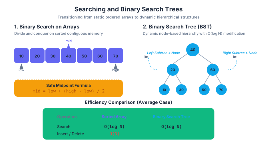
To implement binary search correctly, one must maintain two pointers, low and high, representing the current bounds of the search.
- Calculate the midpoint:
mid = low + (high - low) / 2. - Compare
array[mid]with thetarget. - If
array[mid] == target, returnmid. - If
target < array[mid], sethigh = mid - 1. - If
target > array[mid], setlow = mid + 1.
Mathematical Analysis
The efficiency of binary search is derived from the fact that the search area is halved at each step. If we have $N$ elements, after $k$ steps, we have $N/2^k$ elements remaining. The search terminates when $N/2^k = 1$, which implies $k = \log_2 N$.
| Metric | Complexity | Description |
|---|---|---|
| Best Case | $O(1)$ | The middle element is the target. |
| Average Case | $O(\log N)$ | Standard logarithmic performance. |
| Worst Case | $O(\log N)$ | Target is at the ends or not present. |
| Space Complexity | $O(1)$ | Iterative implementation uses constant space. |
Common Pitfall: The Midpoint Overflow
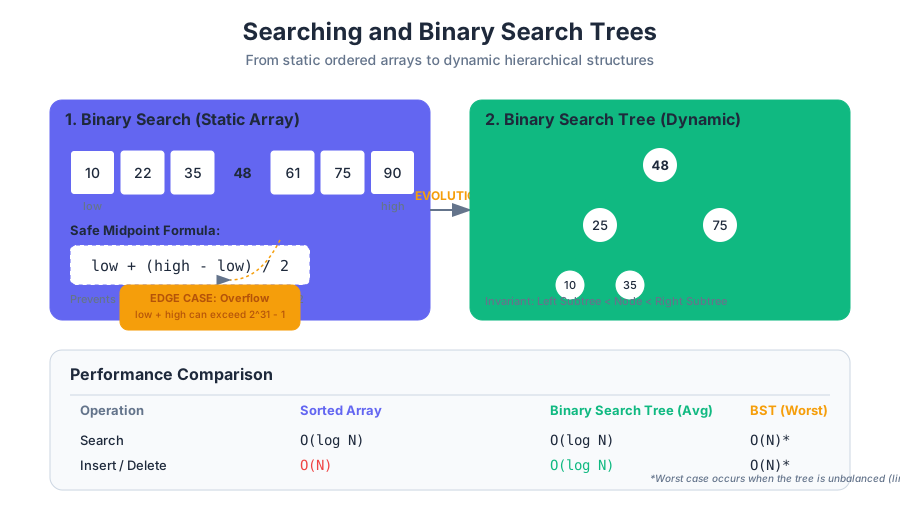
A classic bug in binary search is calculating the midpoint as (low + high) / 2. In many programming languages, if low + high exceeds the maximum value of a signed 32-bit integer, it will overflow to a negative number, causing an index out of bounds error. The robust way to write this is low + (high - low) / 2.
Binary Search Trees (BST)
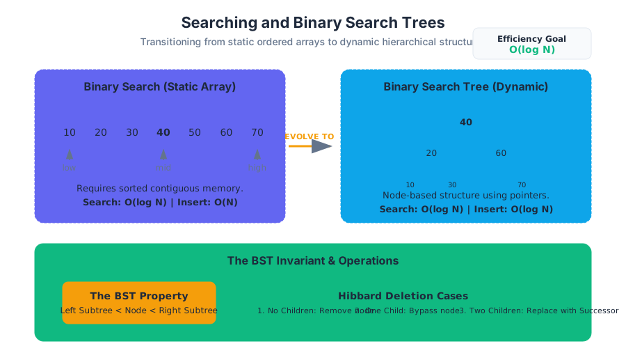
While binary search is exceptionally fast, it requires the data to be stored in a sorted array. Arrays are "static" structures—inserting or deleting an element requires $O(N)$ time because subsequent elements must be shifted. To achieve $O(\log N)$ for both searching and modification, we move to a dynamic, node-based structure: the Binary Search Tree.
The BST Invariant
A Binary Search Tree is a binary tree where each node follows a specific ordering property:
The BST Property For any given node $X$:
- Every node in the left subtree of $X$ has a key strictly less than $X$'s key.
- Every node in the right subtree of $X$ has a key strictly greater than $X$'s key.
BST Implementation in Java
A typical BST node contains a key, an associated value, and references to its children.
public class BST<Key extends Comparable<Key>, Value> {
    private Node root;

    private class Node {
        private Key key;
        private Value val;
        private Node left, right;
        private int size; // Number of nodes in subtree

        public Node(Key key, Value val, int size) {
            this.key = key;
            this.val = val;
            this.size = size;
        }
    }

    public Value get(Key key) {
        return get(root, key);
    }

    private Value get(Node x, Key key) {
        if (x == null) return null;
        int cmp = key.compareTo(x.key);
        if      (cmp < 0) return get(x.left, key);
        else if (cmp > 0) return get(x.right, key);
        else              return x.val;
    }

    public void put(Key key, Value val) {
        root = put(root, key, val);
    }

    private Node put(Node x, Key key, Value val) {
        if (x == null) return new Node(key, val, 1);
        int cmp = key.compareTo(x.key);
        if      (cmp < 0) x.left  = put(x.left,  key, val);
        else if (cmp > 0) x.right = put(x.right, key, val);
        else              x.val   = val;
        x.size = 1 + size(x.left) + size(x.right);
        return x;
    }
}
BST Operations: Search, Insertion, and Deletion
Search and Insertion
Searching and inserting in a BST follow the same logic as binary search. We compare the target key to the current node and move left or right accordingly. Insertion always happens at a null link (a leaf position), maintaining the tree's structure.
The Challenge of Deletion (Hibbard Deletion)
Deleting a node is significantly more complex because we must maintain the BST invariant after the node is removed. There are three cases:
- Node has no children (Leaf): Simply remove the node.
- Node has one child: Replace the node with its child (bypass the node).
- Node has two children: This is the most difficult case. We must find a replacement node that is larger than everything in the left subtree and smaller than everything in the right subtree. This node is the In-order Successor (the smallest node in the right subtree).
Steps for Case 3:
- Find the node to delete ($t$).
- Find the successor ($x$) of $t$ (the minimum node in $t.right$).
- Delete the minimum from $t.right$ (using a specialized
deleteMinoperation). - Set $x.right$ to the result of the
deleteMinoperation. - Set $x.left$ to $t.left$.
- Replace $t$ with $x$.
| Operation | Average Case | Worst Case (Degenerate) |
|---|---|---|
| Search | $O(\log N)$ | $O(N)$ |
| Insert | $O(\log N)$ | $O(N)$ |
| Delete | $O(\sqrt{N})$* | $O(N)$ |
*Note: Hibbard deletion is known to slightly degrade tree balance over many operations, leading to a $\sqrt{N}$ height in some theoretical models, though $O(\log N)$ is often cited for random insertions.
Tree Traversals
Traversing a tree means visiting every node exactly once. Because trees are non-linear, there are multiple ways to define the "order" of visitation.
Depth-First Search (DFS)
DFS traversals use recursion (or a stack) to go as deep as possible before backtracking.
- In-order (Left, Root, Right): Visits nodes in ascending order. This is the most common traversal for BSTs.
- Pre-order (Root, Left, Right): Useful for creating a copy of the tree or evaluating prefix expressions.
- Post-order (Left, Right, Root): Useful for deleting the tree or evaluating postfix (Reverse Polish) expressions.
Breadth-First Search (BFS)
Also known as Level-order Traversal, this visits nodes level by level, from top to bottom and left to right. This requires a Queue data structure.
| Traversal Type | Order | Primary Use Case |
|---|---|---|
| In-order | L $\to$ Root $\to$ R | Retrieving sorted data from a BST. |
| Pre-order | Root $\to$ L $\to$ R | Serializing a tree structure. |
| Post-order | L $\to$ R $\to$ Root | Postfix math; calculating subtree sizes. |
| Level-order | Level by Level | Finding the shortest path in unweighted graphs. |
Performance Analysis and the "Degenerate" Tree
The power of the BST relies entirely on its height. In a perfectly balanced tree with $N$ nodes, the height is $\sim \log_2 N$. However, the shape of a BST depends entirely on the order of insertion.
The Worst Case: Sequential Insertion
If keys are inserted in sorted order (e.g., 1, 2, 3, 4, 5), the BST becomes a "degenerate" tree—essentially a linked list. In this state, the height $H = N$, and all operations revert to $O(N)$ time complexity.
The Average Case: Random Insertion
If keys are inserted in a random order, the height of the tree is approximately $2 \ln N$ (about $1.39 \log_2 N$). This is the mathematical justification for why BSTs are efficient in practice for most dynamic datasets.
Theorem: BST Height If $N$ distinct keys are inserted into a BST in random order, the expected number of compares for a search hit is $\sim 2 \ln N$.
Comparison of Search Structures
To understand where BSTs fit, we compare them against other fundamental searching methods:
| Structure | Search (Worst) | Insert (Worst) | Ordered Ops? |
|---|---|---|---|
| Sequential Search (Linked List) | $O(N)$ | $O(1)$ | No |
| Binary Search (Sorted Array) | $O(\log N)$ | $O(N)$ | Yes |
| BST (Basic) | $O(N)$ | $O(N)$ | Yes |
| Balanced BST (Red-Black/AVL) | $O(\log N)$ | $O(\log N)$ | Yes |
| Hash Table | $O(1)$* | $O(1)$* | No |
*Amortized average case.
Advanced Context: Balanced Search Trees and Beyond
As noted, the $O(N)$ worst-case for a basic BST is a significant liability for production systems. This led to the development of Balanced Search Trees, such as AVL Trees and Left-Leaning Red-Black Trees (LLRB).
The Core Idea of Balancing
Balanced trees use "rotations" during insertion and deletion to ensure that the height of the tree remains logarithmic regardless of the input order.
- 2-3 Trees: A theoretical construct where nodes can hold one or two keys and have two or three children. They are perfectly balanced.
- Red-Black Trees: A BST representation of a 2-3 tree. They use a "color" bit (Red or Black) on links to represent the 3-nodes of a 2-3 tree.
Connection to Sorting
There is a deep connection between BSTs and QuickSort.
- In QuickSort, the "pivot" acts like the root of a BST.
- The partitioning process in QuickSort is essentially building a BST and then performing an in-order traversal.
- The average-case complexity of both is $O(N \log N)$ for sorting and $O(\log N)$ for searching because they share the same underlying mathematical distribution.
Common Pitfalls and Best Practices
- Ignoring the Invariant: When manually modifying a tree (in an exam or a low-level implementation), always double-check that every node in the left subtree is smaller than the parent. A single misplaced node breaks the $O(\log N)$ search guarantee.
- Recursive Stack Overflow: For very deep, unbalanced trees, recursive
get()orput()calls can lead to aStackOverflowError. In production environments with potentially skewed data, iterative implementations or balanced trees are preferred. - Successor vs. Predecessor: In Hibbard deletion, you can use either the in-order successor (smallest in right subtree) or the in-order predecessor (largest in left subtree). Both are valid, but you must be consistent to avoid structural bias.
- Null Checks: Always handle the
nullcase in recursive methods. The base case for almost every BST algorithm isif (node == null).
Source Materials
Study Data Structures and Algorithmic Analysis on Lykke
This course page is free to open: signed out, you can read its first two sections, and signing in, on any plan, opens the rest. The free Lykke Chrome extension syncs your own Canvas courses, so ChatGPT, Claude and Muse can answer from your classes and deadlines. It only reads Canvas.
Add the free extensionSign in to open every sectionAll sections of Data Structures and Algorithmic Analysis · Browse more course pages