From the free course Data Structures and Algorithmic Analysis on Lykke
Directed Graphs and Shortest Paths
Key concepts: Directed Graphs (Digraphs) · Adjacency Lists · Dijkstra's Algorithm · Edge Relaxation
Modeling complex relationships using graphs and finding the most efficient paths between nodes.
Directed Graphs and Shortest Paths
The study of graphs is the study of relationships. While undirected graphs model symmetric relationships—like a physical cable connecting two routers—many real-world systems are inherently asymmetric. A one-way street, a hyperlink from one webpage to another, or a prerequisite requirement for a university course all possess a specific directionality. These are Directed Graphs, or Digraphs.
In this deep dive, we will explore the formal structure of digraphs, the efficiency of various representation methods, and the algorithmic crown jewel of graph theory: Dijkstra’s Algorithm. We will move beyond simple definitions to understand the mathematical mechanics of Edge Relaxation and the data structure optimizations that allow these algorithms to scale to the size of the modern internet.
The Anatomy of Directed Graphs (Digraphs)
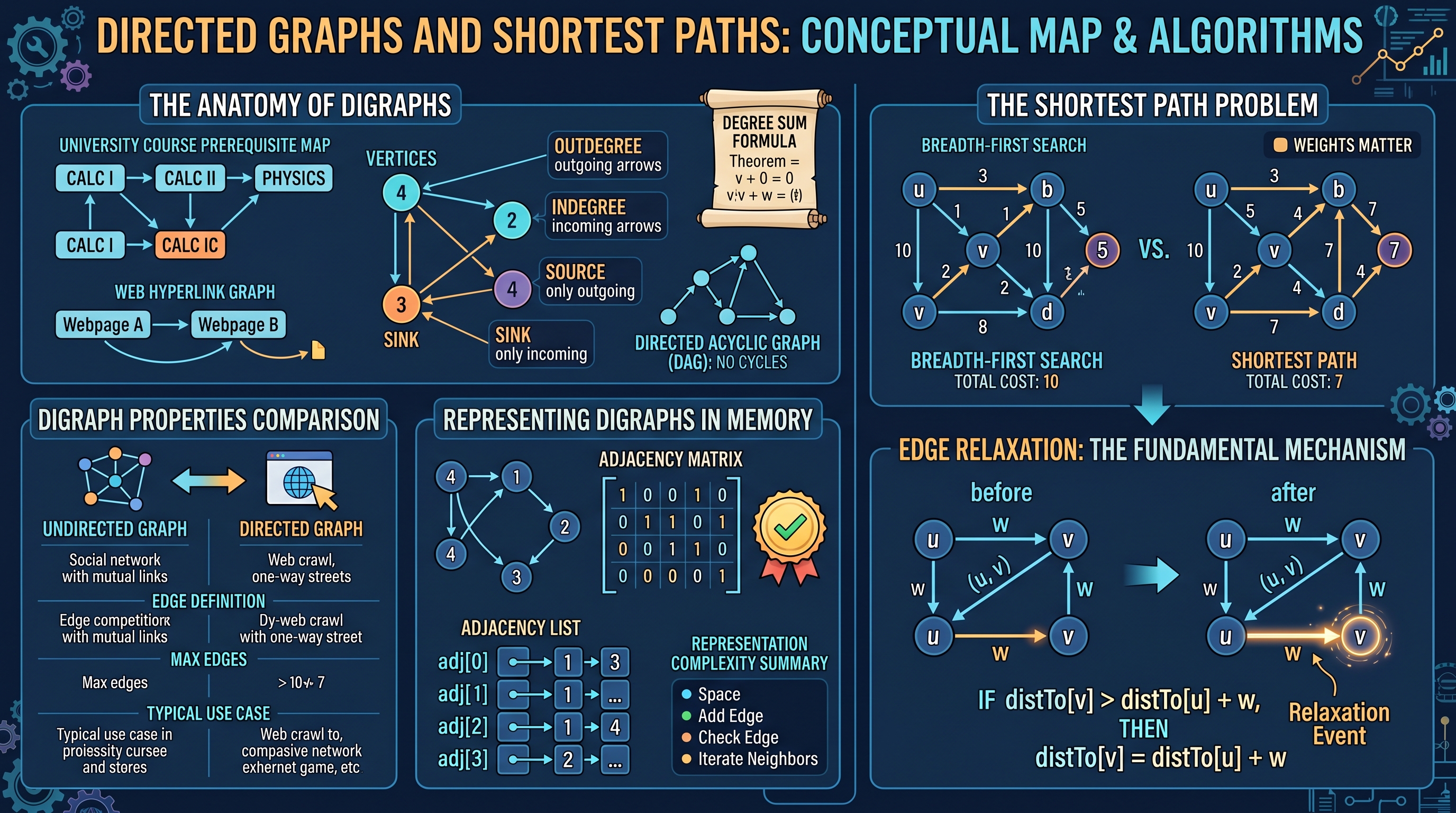
A Directed Graph (Digraph) is a set of vertices $V$ and a set of directed edges $E$. Each edge is an ordered pair of vertices $(u, v)$, representing a path from $u$ to $v$. Unlike undirected graphs, the existence of an edge $(u, v)$ does not imply the existence of $(v, u)$.
Formal Definitions and Terminology
To discuss digraphs with precision, we must define the metrics of connectivity:
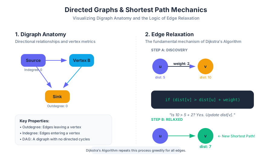
- Outdegree: The number of edges leaving a vertex.
- Indegree: The number of edges entering a vertex.
- Source: A vertex with an indegree of 0.
- Sink: A vertex with an outdegree of 0.
- Strong Connectivity: A digraph is strongly connected if there is a directed path between every pair of vertices.
- Directed Acyclic Graph (DAG): A digraph containing no directed cycles. These are fundamental for modeling dependencies and scheduling.
Theorem: The Degree Sum Formula for Digraphs In any digraph $G = (V, E)$, the sum of the outdegrees of all vertices is equal to the sum of the indegrees, and both are equal to the total number of edges $|E|$. $$\sum_{v \in V} outdeg(v) = \sum_{v \in V} indeg(v) = |E|$$
Digraph Properties Comparison
| Property | Undirected Graph | Directed Graph (Digraph) |
|---|---|---|
| Edge Definition | Unordered pair ${u, v}$ | Ordered pair $(u, v)$ |
| Connectivity | Connected / Disconnected | Strongly / Weakly Connected |
| Max Edges | $V(V-1)/2$ | $V(V-1)$ |
| Traversal | BFS / DFS | BFS / DFS (Direction-sensitive) |
| Typical Use Case | Social networks, Maps | Web crawls, Task scheduling |
Representing Digraphs in Memory
Choosing the right data structure is a trade-off between memory consumption and the speed of specific queries (e.g., "Is $u$ connected to $v$?").
Adjacency Matrix
An Adjacency Matrix is a 2D array of size $V \times V$. For an unweighted graph, matrix[i][j] is 1 if there is an edge from $i$ to $j$, and 0 otherwise. For weighted graphs, the cell stores the weight value.
- Pros: $O(1)$ time to check if an edge exists.
- Cons: $O(V^2)$ space complexity, which is prohibitive for sparse graphs (where $E \ll V^2$).
Adjacency List
An Adjacency List uses an array of size $V$, where each entry adj[i] points to a linked list or dynamic array of all vertices $j$ such that an edge $(i, j)$ exists.
- Pros: $O(V + E)$ space complexity. Efficient for iterating over neighbors.
- Cons: Checking if a specific edge $(u, v)$ exists takes $O(outdeg(u))$ time.
Representation Complexity Summary
| Operation | Adjacency Matrix | Adjacency List |
|---|---|---|
| Space Complexity | $O(V^2)$ | $O(V + E)$ |
| Add Edge | $O(1)$ | $O(1)$ |
| Check Edge (u, v) | $O(1)$ | $O(outdeg(u))$ |
| Iterate Neighbors of u | $O(V)$ | $O(outdeg(u))$ |
| Suitability | Dense Graphs ($E \approx V^2$) | Sparse Graphs ($E \approx V$) |
The Shortest Path Problem
In a weighted digraph, the Shortest Path from vertex $s$ to vertex $t$ is a directed path such that the sum of the weights of its constituent edges is minimized.
Why Weights Matter
In an unweighted graph, Breadth-First Search (BFS) is sufficient to find the shortest path because "shortest" simply means "fewest edges." However, in real-world scenarios—like calculating the fastest route from New York to Boston—edges have weights representing distance, time, or fuel cost. BFS fails here because a path with three short edges might be "shorter" than a path with one very long edge.
Edge Relaxation: The Fundamental Mechanism
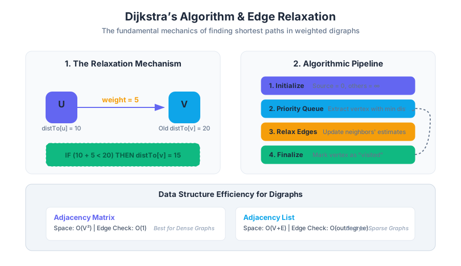
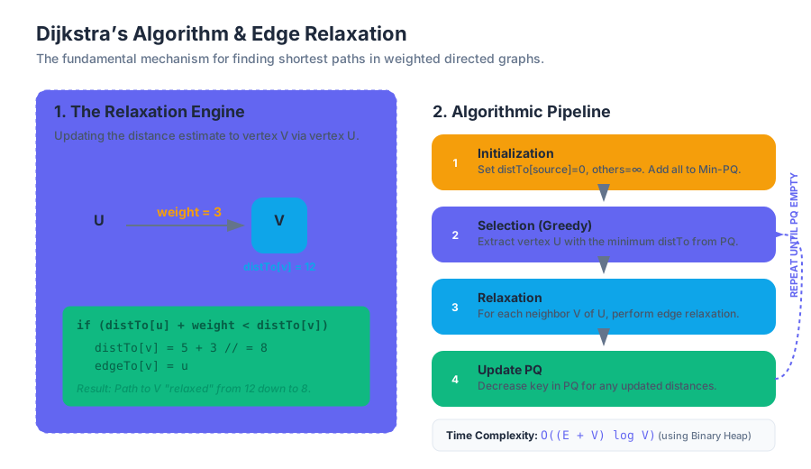
The "engine" of almost every shortest-path algorithm is Relaxation. Imagine you have an estimate of the distance from the start node $s$ to a node $v$, denoted as distTo[v]. If you discover an edge from $u$ to $v$ with weight $w$, you check if going through $u$ provides a shorter path to $v$ than your current estimate.
Definition: Relaxation For an edge $e = (u, v)$ with weight $w$: If
distTo[v] > distTo[u] + w:distTo[v] = distTo[u] + wedgeTo[v] = u
Relaxation "tightens" the distance estimate. We start with all distTo values set to infinity (except the source, which is 0) and repeatedly relax edges until we find the minimum.
Dijkstra’s Algorithm
Developed by Edsger W. Dijkstra in 1956, this algorithm is a Greedy Algorithm that solves the single-source shortest path problem for graphs with non-negative edge weights.
How It Works: The Logic
Dijkstra’s maintains a set of "visited" vertices whose shortest distance from the source is already known. In each iteration, it picks the "unvisited" vertex with the smallest current distance estimate, "visits" it, and relaxes all of its outgoing edges.
- Initialize: Set
distTo[s] = 0anddistTo[v] = ∞for all other vertices. - Priority Queue: Insert all vertices into a Min-Priority Queue (PQ) keyed by their
distTovalue. - Loop: While the PQ is not empty:
- Delete the vertex $u$ with the minimum distance from the PQ.
- For each neighbor $v$ of $u$:
- Relax the edge $(u, v)$.
- If the relaxation decreases
distTo[v], update $v$'s position in the PQ.
Implementation in Java
The following implementation uses an IndexMinPQ, a common structure in textbook implementations (like Sedgewick's) that allows for the decreaseKey operation efficiently.
public class DijkstraSP {
    private double[] distTo;          // distTo[v] = distance of shortest s->v path
    private DirectedEdge[] edgeTo;    // edgeTo[v] = last edge on shortest s->v path
    private IndexMinPQ<Double> pq;    // priority queue of vertices

    public DijkstraSP(EdgeWeightedDigraph G, int s) {
        distTo = new double[G.V()];
        edgeTo = new DirectedEdge[G.V()];

        for (int v = 0; v < G.V(); v++)
            distTo[v] = Double.POSITIVE_INFINITY;
        distTo[s] = 0.0;

        pq = new IndexMinPQ<Double>(G.V());
        pq.insert(s, 0.0);

        while (!pq.isEmpty()) {
            int v = pq.delMin();
            for (DirectedEdge e : G.adj(v))
                relax(e);
        }
    }

    private void relax(DirectedEdge e) {
        int v = e.from(), w = e.to();
        if (distTo[w] > distTo[v] + e.weight()) {
            distTo[w] = distTo[v] + e.weight();
            edgeTo[w] = e;
            if (pq.contains(w)) pq.decreaseKey(w, distTo[w]);
            else                pq.insert(w, distTo[w]);
        }
    }
}
Complexity Analysis of Dijkstra
The efficiency of Dijkstra’s algorithm depends heavily on the data structure used for the Priority Queue.
Complexity Breakdown
| PQ Implementation | insert |
delete-min |
decrease-key |
Total Time Complexity |
|---|---|---|---|---|
| Array | $O(1)$ | $O(V)$ | $O(1)$ | $O(V^2)$ |
| Binary Heap | $O(\log V)$ | $O(\log V)$ | $O(\log V)$ | $O(E \log V)$ |
| Fibonacci Heap | $O(1)$ | $O(\log V)$ | $O(1)$ (amortized) | $O(E + V \log V)$ |
For most practical applications, the Binary Heap (specifically an Indexed Binary Heap) provides the best balance of performance and implementation simplicity. In a sparse graph where $E$ is close to $V$, $E \log V$ is very efficient. In a dense graph where $E \approx V^2$, the simple array implementation $O(V^2)$ can actually be faster due to lower constant factors.
Variations and Extensions
While Dijkstra is the standard, it is not always the best tool for every job.
1. A* Search Algorithm
A* is an extension of Dijkstra used in AI and games. It uses a heuristic $h(v)$ to estimate the distance from $v$ to the goal. The priority queue is keyed by $f(v) = distTo[v] + h(v)$. If the heuristic is "admissible" (never overestimates), A* will find the shortest path much faster by "steering" the search toward the destination.
2. Directed Acyclic Graphs (DAGs)
If a graph is a DAG, we can find the shortest path in $O(V + E)$ time by relaxing vertices in Topological Order. This is even faster than Dijkstra because it doesn't require a priority queue. This method also works for finding the Longest Path in a DAG, which is useful for critical path analysis in project management.
3. Bellman-Ford Algorithm
Dijkstra fails if there are negative edge weights. If a graph has negative weights but no negative cycles, the Bellman-Ford algorithm can find the shortest path in $O(VE)$ time.
Shortest Path Algorithm Comparison
| Algorithm | Restriction | Complexity | Note |
|---|---|---|---|
| BFS | Unweighted edges | $O(V + E)$ | Only for uniform weights |
| Dijkstra | Non-negative weights | $O(E \log V)$ | Standard for most maps |
| DAG Shortest Path | No cycles | $O(V + E)$ | Uses Topological Sort |
| Bellman-Ford | No negative cycles | $O(VE)$ | Handles negative weights |
Common Pitfalls and Edge Cases
The Negative Weight Trap
A common misconception is that you can "fix" negative weights by adding a large constant to every edge weight to make them all positive. This does not work. Adding a constant $C$ to every edge penalizes paths with more edges more heavily than paths with fewer edges, potentially changing which path is the shortest.
Cycles and Infinite Loops
In a graph with a negative cycle (a cycle where the sum of weights is less than zero), a "shortest path" does not exist because you could traverse the cycle infinitely many times to achieve a distance of $-\infty$. Dijkstra’s algorithm will not detect this; it will simply produce an incorrect result. Bellman-Ford is required to detect negative cycles.
Floating Point Precision
When weights are floating-point numbers (doubles), cumulative rounding errors can occur. In high-stakes financial or scientific applications, it is often better to use integers (e.g., representing dollars as cents) to maintain precision.
Performance in Dense Graphs
In a complete graph where $E = V(V-1)$, Dijkstra’s $O(E \log V)$ becomes $O(V^2 \log V)$. In this specific case, using a simple array for the priority queue—which results in $O(V^2)$—is mathematically and practically superior.
Summary of the Shortest Path Pipeline
To solve a shortest path problem in a production environment, an engineer typically follows this pipeline:
- Identify the Graph Type: Is it directed? Are there cycles?
- Validate Weights: Are there negative weights? If yes, use Bellman-Ford. If no, proceed.
- Check for DAG structure: If it's a DAG, use Topological Sort for $O(V+E)$ performance.
- Select Data Structure: For general graphs, use Dijkstra with an Indexed Binary Heap.
- Relaxation: Iterate through the graph, relaxing edges and updating the Priority Queue until the sink is reached or the PQ is empty.
- Path Reconstruction: Use the
edgeTo[]array to backtrack from the destination to the source to retrieve the actual path.
Source Materials
Study Data Structures and Algorithmic Analysis on Lykke
This course page is free to open: signed out, you can read its first two sections, and signing in, on any plan, opens the rest. The free Lykke Chrome extension syncs your own Canvas courses, so ChatGPT, Claude and Muse can answer from your classes and deadlines. It only reads Canvas.
Add the free extensionSign in to open every sectionAll sections of Data Structures and Algorithmic Analysis · Browse more course pages