From the free course Data Structures and Algorithmic Analysis on Lykke
Union-Find and Big O Analysis
Key concepts: Big O Notation · Dynamic Connectivity · Quick-Find · Quick-Union · Weighted Quick-Union
Introduction to algorithmic efficiency and the dynamic connectivity problem using Union-Find algorithms.
Union-Find and Big O Analysis
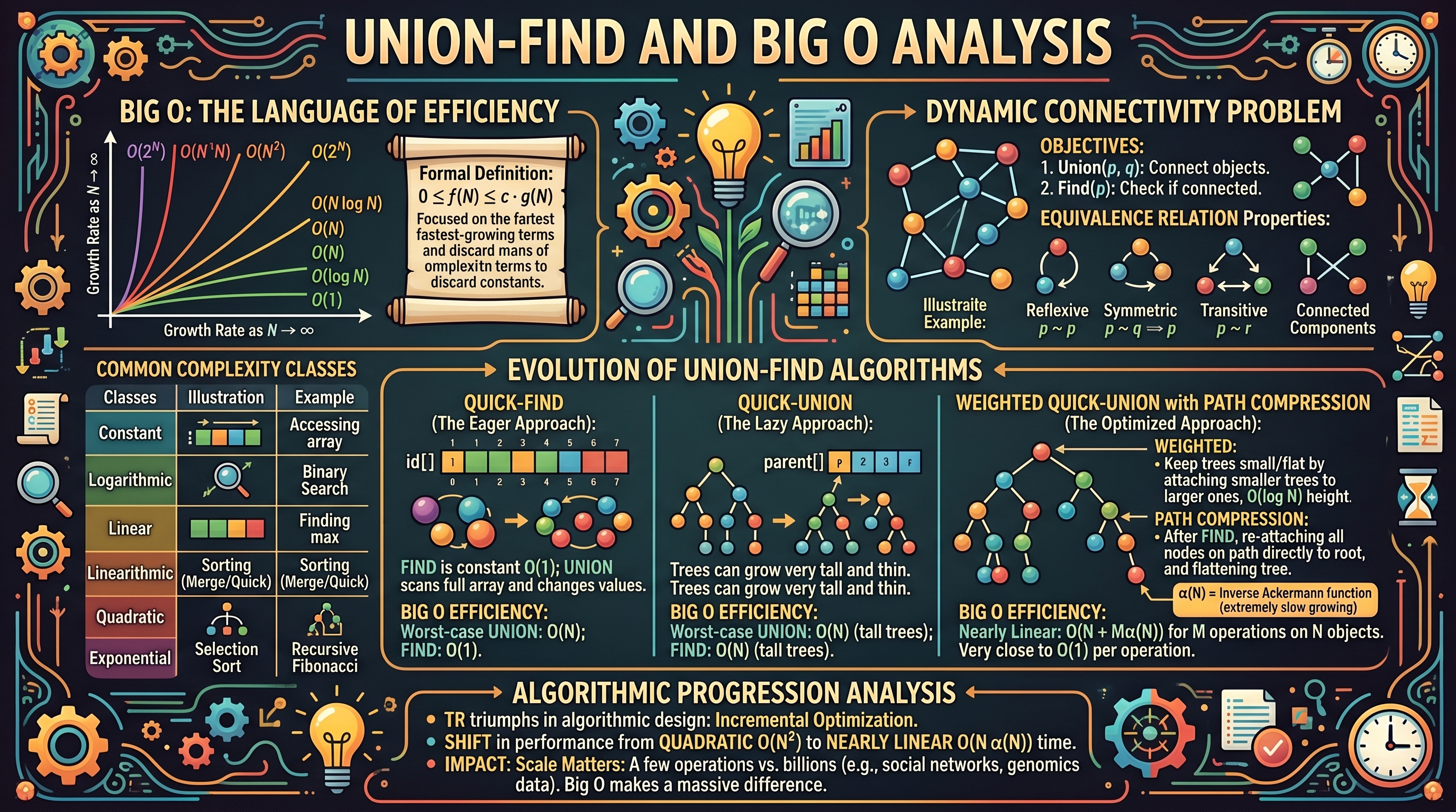
The study of algorithms is inextricably linked to the study of efficiency. In the realm of computer science, we are rarely concerned with whether a problem can be solved—given enough time and memory, most computable problems can be—but rather whether it can be solved within the constraints of reality. This article explores the symbiotic relationship between Big O Analysis, the mathematical language of efficiency, and Union-Find, a sophisticated data structure designed to solve the Dynamic Connectivity problem.
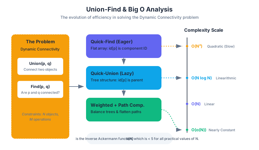
At its core, Union-Find represents a triumph of incremental optimization. By evolving a simple, "eager" approach into a "lazy," weighted, and flattened structure, we can observe a dramatic shift in computational complexity from quadratic time to nearly linear time. This progression serves as a masterclass in algorithmic design and the practical application of asymptotic analysis.
The Foundation: Big O Notation and Complexity Analysis
Before diving into specific data structures, we must establish the framework for measurement. Big O Notation provides a theoretical upper bound on the execution time or space requirements of an algorithm as the input size $N$ grows toward infinity. It allows us to ignore hardware-specific constants and focus on the order of growth.
The Formal Definition
Definition: A function $f(N)$ is $O(g(N))$ if there exist positive constants $c$ and $N_0$ such that $0 \le f(N) \le c \cdot g(N)$ for all $N \ge N_0$.
In practice, this means we focus on the fastest-growing term and discard coefficients. For instance, an algorithm that performs $5N^2 + 20N + 100$ operations is categorized as $O(N^2)$. As $N$ becomes massive, the $N^2$ term dominates the total execution time, rendering the $20N$ and constant $100$ negligible.
Common Complexity Classes
| Notation | Name | Description | Example |
|---|---|---|---|
| $O(1)$ | Constant | Time does not change with input size. | Accessing an array index. |
| $O(\log N)$ | Logarithmic | Time increases slowly; doubling $N$ adds a constant step. | Binary Search. |
| $O(N)$ | Linear | Time is directly proportional to input size. | Finding the max in an unsorted list. |
| $O(N \log N)$ | Linearithmic | Slightly worse than linear; standard for efficient sorting. | Merge Sort, Quick Sort. |
| $O(N^2)$ | Quadratic | Time grows with the square of $N$; often involves nested loops. | Selection Sort, Quick-Find Union. |
| $O(2^N)$ | Exponential | Time doubles with each addition to $N$; computationally expensive. | Recursive Fibonacci. |
Why Big O Matters in Union-Find
The Dynamic Connectivity problem involves a set of $N$ objects. We perform $M$ union operations. If our algorithm is $O(N)$, and we do $M$ operations, the total time is $O(MN)$. If $M$ and $N$ are both $10^9$ (a common scale for social networks or genomic data), a quadratic algorithm would take $10^{18}$ operations. On a standard processor, this would take decades. An $O(\log N)$ or $O(\alpha(N))$ algorithm, however, would finish in seconds.
The Dynamic Connectivity Problem
The Union-Find data structure (also known as a Disjoint Set Union or DSU) is designed to solve the dynamic connectivity problem. Given a set of $N$ objects, we need to support two primary operations:
- Union: Connect two objects.
- Find (or Connected): Determine if there is a path connecting two objects.
We assume "connected" is an equivalence relation, meaning it is:
- Reflexive: $p$ is connected to $p$.
- Symmetric: If $p$ is connected to $q$, then $q$ is connected to $p$.
- Transitive: If $p$ is connected to $q$ and $q$ is connected to $r$, then $p$ is connected to $r$.
These properties allow us to partition the objects into connected components. A connected component is a maximal set of objects that are all mutually connected.
Quick-Find: The Eager Approach
Quick-Find is the most intuitive implementation of Union-Find. It prioritizes the speed of the find operation.
How it Works
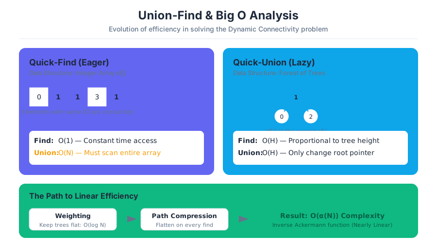
We maintain an integer array id[] of size $N$. If id[p] is equal to id[q], then $p$ and $q$ are in the same component.
- Find: Simply check if
id[p] == id[q]. This is a constant time $O(1)$ operation. - Union: To merge components containing $p$ and $q$, we must change all entries whose value is
id[p]toid[q].
Implementation (Java)
public class QuickFindUF {
    private int[] id;

    public QuickFindUF(int N) {
        id = new int[N];
        for (int i = 0; i < N; i++) id[i] = i;
    }

    public boolean connected(int p, int q) {
        return id[p] == id[q];
    }

    public void union(int p, int q) {
        int pid = id[p];
        int qid = id[q];
        for (int i = 0; i < id.length; i++) {
            if (id[i] == pid) id[i] = qid;
        }
    }
}
Analysis of Quick-Find
While find is incredibly fast, union is prohibitively expensive. To perform $N$ union operations on $N$ objects, the time complexity is $O(N^2)$.
| Operation | Complexity |
|---|---|
| Initialize | $O(N)$ |
| Union | $O(N)$ |
| Find | $O(1)$ |
The Pitfall: Quick-Find is "eager." It does too much work during the union step to ensure the find step is easy. In a world of Big Data, $O(N^2)$ is effectively non-computable for large $N$.
Quick-Union: The Lazy Approach
To address the $O(N)$ union cost, Quick-Union adopts a "lazy" strategy. Instead of updating every element in a component, we represent components as trees.
How it Works
The id[] array now stores the parent of each element.
- Find: To find the component of $p$, follow parent pointers until you reach a root (where
id[i] == i). - Union: To merge components containing $p$ and $q$, find their respective roots and set the root of $p$ to point to the root of $q$.
Implementation (Java)
public class QuickUnionUF {
    private int[] id;

    public QuickUnionUF(int N) {
        id = new int[N];
        for (int i = 0; i < N; i++) id[i] = i;
    }

    private int root(int i) {
        while (i != id[i]) i = id[i];
        return i;
    }

    public boolean connected(int p, int q) {
        return root(p) == root(q);
    }

    public void union(int p, int q) {
        int i = root(p);
        int j = root(q);
        id[i] = j;
    }
}
Analysis of Quick-Union
Quick-Union speeds up the union operation (assuming we already have the roots), but it introduces a new problem: tree height. In the worst case, the trees can become very tall (a "skinny" tree or a linked list). If the tree height is $N$, then both find and union become $O(N)$.
| Operation | Complexity (Worst Case) |
|---|---|
| Initialize | $O(N)$ |
| Union | $O(N)$ (includes finding roots) |
| Find | $O(N)$ |
Weighted Quick-Union: Balancing the Trees
The primary weakness of Quick-Union is that we might accidentally attach a large tree to the root of a small tree, increasing the overall height. Weighted Quick-Union solves this by always attaching the smaller tree to the root of the larger tree.
The Mechanics
We maintain an additional array sz[] to keep track of the number of objects in each tree.
- Find the roots of $p$ and $q$.
- Compare the sizes of the trees rooted at $p$ and $q$.
- Connect the root of the smaller tree to the root of the larger tree.
- Update the
sz[]array for the new root.
Implementation (Java)
public class WeightedQuickUnionUF {
    private int[] id;
    private int[] sz;

    public WeightedQuickUnionUF(int N) {
        id = new int[N];
        sz = new int[N];
        for (int i = 0; i < N; i++) {
            id[i] = i;
            sz[i] = 1;
        }
    }

    private int root(int i) {
        while (i != id[i]) i = id[i];
        return i;
    }

    public void union(int p, int q) {
        int i = root(p);
        int j = root(q);
        if (i == j) return;
        if (sz[i] < sz[j]) { id[i] = j; sz[j] += sz[i]; }
        else               { id[j] = i; sz[i] += sz[j]; }
    }
}
Mathematical Proof of $O(\log N)$
The depth of any node $x$ is at most $\lg N$ (log base 2 of $N$).
Proof: When does the depth of $x$ increase? The depth of $x$ increases by 1 only when the tree $T_1$ containing $x$ is merged into another tree $T_2$. According to our algorithm, this only happens if $size(T_2) \ge size(T_1)$. When this happens, the size of the new tree containing $x$ is $size(T_1) + size(T_2)$, which is at least $2 \times size(T_1)$. In other words, every time the depth of $x$ increases, the size of its tree at least doubles. How many times can the size of a tree containing $N$ nodes double? At most $\lg N$ times. Therefore, the depth of any node is capped at $\lg N$.
| Operation | Complexity |
|---|---|
| Initialize | $O(N)$ |
| Union | $O(\log N)$ |
| Find | $O(\log N)$ |
Path Compression: Flattening the Structure
Even with weighting, we can improve performance further. Path Compression ensures that trees stay almost completely flat by re-linking nodes directly to the root during the find operation.
How it Works
When looking for the root of $p$, we can make every other node in the path point to its grandparent, effectively halving the path length. This is a "one-pass" implementation. A "two-pass" implementation would make every node on the path point directly to the root.
private int root(int i) {
    while (i != id[i]) {
        id[i] = id[id[i]]; // One-pass path compression
        i = id[i];
    }
    return i;
}
The Inverse Ackermann Function
When you combine Weighted Quick-Union with Path Compression, the amortized time per operation is $O(\alpha(N))$, where $\alpha$ is the Inverse Ackermann function. For all practical values of $N$ (up to the number of atoms in the observable universe), $\alpha(N) < 5$. This makes the algorithm effectively constant time in practice, though theoretically it is slightly more than constant.
Comparative Analysis of Union-Find Variants
The following table summarizes the performance of the different approaches we have discussed. Note how the complexity shifts from $N$ to $\log N$ and finally to nearly constant time.
| Algorithm | Constructor | Union | Find | Total Time ($M$ unions on $N$ objects) |
|---|---|---|---|---|
| Quick-Find | $N$ | $N$ | $1$ | $MN$ |
| Quick-Union | $N$ | $N^\dagger$ | $N$ | $MN$ |
| Weighted QU | $N$ | $\log N$ | $\log N$ | $N + M \log N$ |
| QU + Path Comp | $N$ | $\log N$ | $\log N$ | $N + M \log N$ |
| WQU + Path Comp | $N$ | $\alpha(N)$ | $\alpha(N)$ | $N + M \alpha(N)$ |
$^\dagger$ Note: Quick-Union's union operation is $O(N)$ because it is dominated by the cost of finding the roots in a tall tree.
Practical Performance Example
Consider a scenario with $N = 10^9$ objects and $M = 10^9$ union operations.
| Algorithm | Operations (Approximate) | Real-world Time (Estimate) |
|---|---|---|
| Quick-Find | $10^{18}$ | ~30 years |
| Weighted QU | $3 \times 10^{10}$ | ~30 seconds |
| WQU + Path Comp | $5 \times 10^9$ | ~6 seconds |
Common Pitfalls and Edge Cases
- Union of Already Connected Elements: A common mistake is failing to check if
root(p) == root(q)before performing a union. In Weighted Quick-Union, failing to do this will result in incorrectly incrementing the size of the component. - Path Compression in Union: Path compression should be implemented inside the
root()orfind()method, not theunion()method. This ensures that every time a node is accessed, the tree is flattened. - Memory Constraints: For $N = 10^9$, the
id[]andsz[]arrays (assuming 4-byte integers) would require roughly 8GB of RAM. In memory-constrained environments, one might need to use a more compact representation or a hash-map-based approach if the set is sparse. - Misunderstanding $\alpha(N)$: Students often confuse $O(\alpha(N))$ with $O(1)$. While they are practically the same, $\alpha(N)$ is technically growing. On an exam, stating Union-Find is $O(1)$ without the "amortized" or "Inverse Ackermann" qualifier may be considered technically incorrect.
Applications of Union-Find
The efficiency of Union-Find makes it a staple in several high-level algorithms and systems:
- Percolation Theory: Used in physics and chemistry to model the flow of liquids through porous media. We use Union-Find to determine if a system "percolates" (has a path from top to bottom).
- Kruskal’s Minimum Spanning Tree: A greedy algorithm that uses Union-Find to detect cycles as it adds edges to a graph.
- Image Processing: In "Connected Component Labeling," Union-Find identifies clusters of similar pixels to distinguish objects in an image.
- Network Connectivity: Determining if two computers in a massive network can communicate or if two people in a social network are in the same "friend circle."
Summary of Big O and Union-Find
The journey from Quick-Find to Weighted Quick-Union with Path Compression illustrates the core philosophy of algorithmic optimization. By analyzing the Big O of our initial approach, we identified a bottleneck (the $O(N)$ union). By changing our perspective from an eager array to a lazy tree structure, and then applying mathematical balancing and path flattening, we reduced the complexity to a level where problems of nearly infinite scale become trivial.
Source Materials
Study Data Structures and Algorithmic Analysis on Lykke
This course page is free to open: signed out, you can read its first two sections, and signing in, on any plan, opens the rest. The free Lykke Chrome extension syncs your own Canvas courses, so ChatGPT, Claude and Muse can answer from your classes and deadlines. It only reads Canvas.
Add the free extensionSign in to open every sectionAll sections of Data Structures and Algorithmic Analysis · Browse more course pages