From the free course Data Structures and Algorithmic Analysis on Lykke
Balanced Search Trees
Key concepts: Tree Balance · AVL Trees · Red-Black Trees · Rotations
Advanced tree structures designed to maintain logarithmic height and guarantee performance.
Balanced Search Trees
Overview
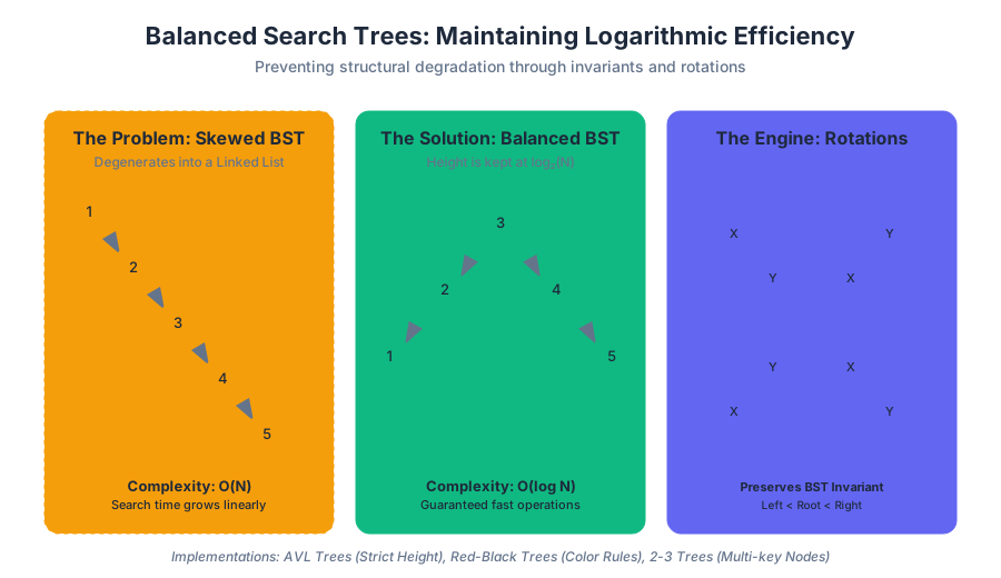
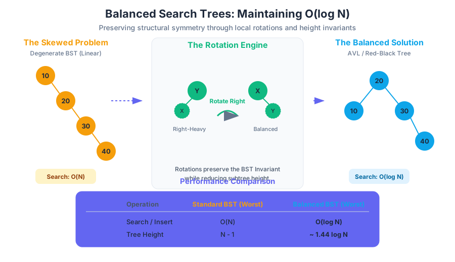
In the realm of computer science, the Binary Search Tree (BST) is a fundamental data structure designed to facilitate fast searching, insertion, and deletion. However, the efficiency of a BST is inextricably linked to its shape. A standard BST offers no guarantees regarding its structural symmetry; if keys are inserted in a sorted or semi-sorted order, the tree "skews," collapsing into a structure functionally identical to a linked list. This transformation degrades the time complexity of core operations from $O(\log N)$ to $O(N)$.
Balanced Search Trees solve this structural fragility by enforcing strict invariants. Through the use of local transformations called rotations and specific coloring or height-tracking rules, these trees ensure that the height $h$ remains logarithmic relative to the number of nodes $N$. This section explores the mechanics of balance, focusing on the two most prominent implementations: AVL Trees and Red-Black Trees.
The Balance Problem: From Logarithmic to Linear
The primary motivation for balancing a tree is the preservation of the Logarithmic Guarantee. In a perfectly balanced binary tree, the path from the root to any leaf is approximately $\log_2 N$.
The Height Theorem: For any binary tree with $N$ nodes and height $h$:
- The minimum height is $\lfloor \log_2 N \rfloor$.
- The maximum height is $N-1$ (a degenerate tree).
- The search time is proportional to the height: $O(h)$.
If we insert the keys [1, 2, 3, 4, 5] into a standard BST, we obtain a "right-leaning" chain. Every search for the value 5 requires five comparisons. In a balanced version, the same keys would result in a tree of height 2, requiring at most three comparisons.
Performance Comparison: BST vs. Balanced BST
| Operation | Average BST | Worst-case BST (Skewed) | Balanced BST (Worst-case) |
|---|---|---|---|
| Search | $O(\log N)$ | $O(N)$ | $O(\log N)$ |
| Insert | $O(\log N)$ | $O(N)$ | $O(\log N)$ |
| Delete | $O(\log N)$ | $O(N)$ | $O(\log N)$ |
| Space | $O(N)$ | $O(N)$ | $O(N)$ |
Tree Rotations: The Engine of Balance
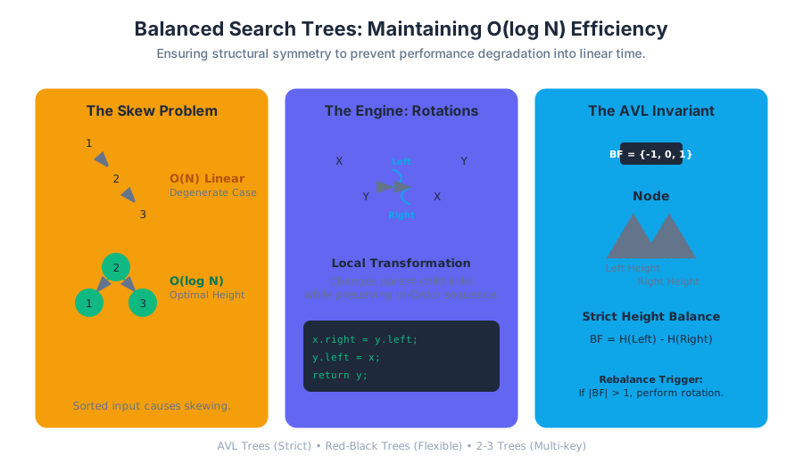
To maintain balance without violating the BST Invariant (where for any node $x$, all keys in the left subtree are smaller than $x$ and all keys in the right subtree are larger), we use Rotations. A rotation is a local algebraic transformation that changes the parent-child relationship of a small group of nodes while preserving their relative in-order sequence.
Left Rotation (Rotate Left)
When a node $x$ has a right child $y$ that is "too heavy," we rotate $x$ to the left. $y$ becomes the new root of this subtree, and $x$ becomes the left child of $y$. If $y$ had a left child $T2$, it is reassigned as the right child of $x$.
Right Rotation (Rotate Right)
The inverse of the left rotation. If a node $y$ has a left child $x$ that is "too heavy," we rotate $y$ to the right. $x$ becomes the new root, and $y$ becomes the right child of $x$.
Rotation Implementation (Java)
private Node rotateRight(Node h) {
    // h is the node that is unbalanced to the left
    Node x = h.left;
    h.left = x.right;
    x.right = h;
    // Update metadata (height or color) here
    return x; // x is the new root of this subtree
}

private Node rotateLeft(Node h) {
    // h is the node that is unbalanced to the right
    Node x = h.right;
    h.right = x.left;
    x.left = h;
    // Update metadata (height or color) here
    return x; // x is the new root of this subtree
}
AVL Trees: Strict Height Balancing
Named after inventors Adelson-Velsky and Landis, the AVL tree was the first dynamically balanced data structure. It maintains balance by tracking the Balance Factor of every node.
The AVL Invariant: For every node in the tree, the height of the left and right subtrees can differ by at most one. $$\text{Balance Factor } (BF) = \text{height}(\text{left_subtree}) - \text{height}(\text{right_subtree})$$ A node is "balanced" if $BF \in {-1, 0, 1}$.
Rebalancing the AVL Tree
When an insertion or deletion causes a node's $BF$ to become $2$ or $-2$, a rebalancing operation is triggered. There are four distinct cases based on where the imbalance originated:
| Case | Condition | Rotation Required |
|---|---|---|
| Left-Left (LL) | New node in left-child's left-subtree | Single Right Rotation |
| Right-Right (RR) | New node in right-child's right-subtree | Single Left Rotation |
| Left-Right (LR) | New node in left-child's right-subtree | Double Rotation (Left then Right) |
| Right-Left (RL) | New node in right-child's left-subtree | Double Rotation (Right then Left) |
Worked Example: AVL Insertion
- Insert 30, 20, 10:
- 30 is root.
- 20 is left child of 30.
- 10 is left child of 20.
- Node 30 now has $BF = 2$. This is a Left-Left case.
- Action: Rotate 30 to the right. 20 becomes the root, 10 and 30 are its children. Height is now 1.
- Insert 25:
- 25 is the left child of 30.
- Tree is still balanced.
- Insert 28:
- 28 is the right child of 25.
- Node 30 now has $BF = 2$ (left height 2, right height 0). The path to the imbalance is Left (25) then Right (28). This is a Left-Right case.
- Action: Rotate 25 left, then rotate 30 right.
2-3 Search Trees: The Theoretical Ideal
Before diving into Red-Black trees, one must understand the 2-3 Tree. Unlike a binary tree, a 2-3 tree allows a node to hold more than one key.
- 2-node: One key, two children (standard BST node).
- 3-node: Two keys, three children.
- Perfect Balance Property: Every path from the root to a null link is exactly the same length.
How 2-3 Trees Grow
Instead of adding a new leaf at the bottom (which would increase height), a 2-3 tree inserts the new key into an existing leaf, temporarily creating a 4-node (3 keys, 4 children). This 4-node then "splits," sending its middle key up to the parent. If the parent becomes a 4-node, it splits again. This process ensures the tree only grows "upward" from the root, maintaining perfect balance.
Red-Black Trees: The Practical Standard
While 2-3 trees are theoretically elegant, they are difficult to implement because of the multiple node types. Red-Black Trees (specifically Left-Leaning Red-Black Trees or LLRBs) are a way to represent 2-3 trees using only standard binary nodes.
The Red-Black Mapping:
- A 2-node in a 2-3 tree is a standard black node in an RB tree.
- A 3-node in a 2-3 tree is represented as two binary nodes connected by a red link. By convention, the red link leans to the left.
Red-Black Properties
To be a valid Red-Black Tree, the following rules must hold:
- Every node is either Red or Black.
- The root is always Black.
- New insertions always start as Red.
- No two Red nodes can be adjacent (no Red child of a Red parent).
- Black Balance: Every path from the root to a null link must contain the same number of Black nodes.
Red-Black Operations
When inserting into an LLRB, we maintain balance using three primary tools:
- Rotate Left: Used to fix a right-leaning red link.
- Rotate Right: Used to fix two consecutive red links.
- Color Flip: Used to split a "4-node" (where both children are red).
private Node put(Node h, Key key, Value val) {
    if (h == null) return new Node(key, val, RED);

    int cmp = key.compareTo(h.key);
    if      (cmp < 0) h.left  = put(h.left,  key, val);
    else if (cmp > 0) h.right = put(h.right, key, val);
    else              h.val   = val;

    // 1. Right-leaning red link? Rotate left.
    if (isRed(h.right) && !isRed(h.left))      h = rotateLeft(h);
    // 2. Two red links in a row? Rotate right.
    if (isRed(h.left)  && isRed(h.left.left)) h = rotateRight(h);
    // 3. Both children red? Flip colors.
    if (isRed(h.left)  && isRed(h.right))     flipColors(h);

    return h;
}
AVL vs. Red-Black: Which to Choose?
Both structures provide $O(\log N)$ performance, but they are optimized for different workloads.
| Feature | AVL Tree | Red-Black Tree |
|---|---|---|
| Balance Strictness | Very Strict ($h < 1.44 \log N$) | Loose ($h < 2 \log N$) |
| Search Speed | Faster (due to flatter structure) | Slightly Slower |
| Insertion/Deletion | Slower (more rotations to maintain strictness) | Faster (fewer rotations) |
| Memory Overhead | Stores height (int) per node | Stores color (1 bit) per node |
| Common Use Case | Read-heavy lookups (Databases) | General purpose (Java TreeMap, C++ std::map) |
Common Pitfalls and Edge Cases
1. Forgetting the Root Color
In Red-Black trees, after any operation, the root must be explicitly set to Black. A red root doesn't necessarily break the structure, but it violates the formal definition and can lead to logic errors in complex deletions.
2. The "Double Rotation" Trap
In AVL trees, beginners often try to fix an LR (Left-Right) imbalance with a single rotation. This is impossible. A single rotation will simply move the imbalance to a different node. You must rotate the child first to convert the case into an LL (Left-Left) case, then rotate the parent.
3. Complexity of Deletion
While insertion in balanced trees is relatively straightforward, deletion is significantly more complex. In Red-Black trees, deletion often involves "Double Black" nodes and up to six different transformation cases. Most production-grade libraries use the "Bottom-Up" insertion but often implement deletion using specific "Top-Down" 2-3-4 tree logic to simplify the code.
4. Precision in Height Calculation
In AVL implementations, failing to update the height of a node after its children have been rotated is a common source of infinite loops or silent balance degradation. The height update must happen from the bottom up as the recursion unwinds.
Key Insight: The beauty of Balanced Search Trees lies in their ability to turn the "luck of the draw" (the order of input data) into a mathematical certainty. By spending a small, constant amount of time $(O(1))$ on rotations during an update, we protect the system against the catastrophic $O(N)$ failure mode.
Source Materials
Study Data Structures and Algorithmic Analysis on Lykke
This course page is free to open: signed out, you can read its first two sections, and signing in, on any plan, opens the rest. The free Lykke Chrome extension syncs your own Canvas courses, so ChatGPT, Claude and Muse can answer from your classes and deadlines. It only reads Canvas.
Add the free extensionSign in to open every sectionAll sections of Data Structures and Algorithmic Analysis · Browse more course pages