From the free course CS323: Numerical Analysis and Computing on Lykke
Root Finding for Nonlinear Equations
Key concepts: Root-Finding · Bisection Method · Fixed-Point Iteration · Newton's Method · Secant Method · Order of Convergence (Linear vs. Quadratic)
This section introduces iterative algorithms for solving nonlinear equations of the form f(x)=0, a common problem known as root-finding. It details and compares several fundamental methods, including the Bisection Method, Fixed-Point Iteration, Newton's Method, and the Secant Method. The focus is on understanding their mechanisms, convergence rates, and practical trade-offs.
Root Finding for Nonlinear Equations
In numerical analysis, while solving systems of linear equations of the form Ax = b is a well-defined and foundational problem, a vast array of challenges in science, engineering, and finance are inherently nonlinear. These problems require us to find the roots (or zeros) of a nonlinear function f(x), which are the values of x such that f(x) = 0. Unlike their linear counterparts, nonlinear equations rarely have a direct, analytical solution. Consequently, we must turn to iterative methods: algorithms that generate a sequence of improving approximations, x_0, x_1, x_2, ..., that—if all goes well—converge to the true root.
The choice of method involves a critical trade-off between speed, robustness, and the amount of information required about the function (such as its derivative). Understanding these algorithms is not just an academic exercise; it's fundamental to solving complex optimization, simulation, and modeling problems.
The Bisection Method: Slow but Steady
The Bisection Method is the simplest and most robust root-finding algorithm. Its reliability stems from a simple, powerful mathematical principle: the Intermediate Value Theorem.
What It Is
The Bisection Method is a bracketing method for finding a root of a continuous function
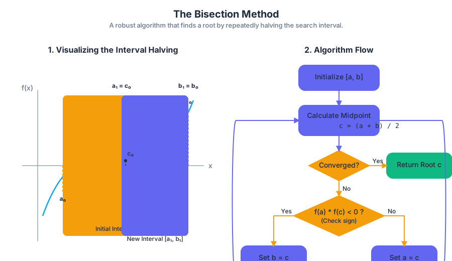
f(x). It begins with an interval[a, b]where the function values at the endpoints,f(a)andf(b), have opposite signs. The method repeatedly halves the interval while ensuring the root remains bracketed within the smaller interval.
The core requirement, f(a) * f(b) < 0, guarantees, by the Intermediate Value Theorem, that at least one root must exist within the interval (a, b).
Why It Matters
The primary virtue of the Bisection Method is its guaranteed convergence. As long as the initial interval brackets a root and the function is continuous, the method will converge to a root. This makes it an excellent fallback or a tool for obtaining a rough but reliable initial guess for a faster, less stable method. Its main drawback is its slow rate of convergence.
How It Works
The algorithm proceeds as follows:
- Initialization: Choose an interval
[a, b]such thatf(a)andf(b)have opposite signs. Define a tolerancetoland a maximum number of iterationsmax_iter. - Iteration: For
n = 1, 2, ...up tomax_iter: a. Calculate the midpoint:c = (a + b) / 2. b. Evaluatef(c). c. Check for convergence: If|f(c)| < tolor(b - a) / 2 < tol, the process has converged. Returnc. d. Update the interval: - Iff(a) * f(c) < 0, the root is in the left half. Setb = c. - Else, the root is in the right half. Seta = c. - Termination: If the loop finishes without converging, the method has failed (e.g.,
max_iterwas reached).
The width of the search interval is halved at each step. After n iterations, the width of the interval containing the root is (b_0 - a_0) / 2^n, where [a_0, b_0] is the initial interval.
Concrete Example
Let's find the root of f(x) = x^3 - x - 2 on the interval [1, 2].
- We know
f(1) = 1 - 1 - 2 = -2andf(2) = 8 - 2 - 2 = 4. Since the signs are opposite, a root is bracketed.
| Iteration (n) | a | b | c = (a+b)/2 | f(c) | New Interval | Interval Width |
|---|---|---|---|---|---|---|
| 1 | 1.0 | 2.0 | 1.5 | -0.125 | [1.5, 2.0] |
0.5 |
| 2 | 1.5 | 2.0 | 1.75 | 1.609375 | [1.5, 1.75] |
0.25 |
| 3 | 1.5 | 1.75 | 1.625 | 0.666016 | [1.5, 1.625] |
0.125 |
| 4 | 1.5 | 1.625 | 1.5625 | 0.252197 | [1.5, 1.5625] |
0.0625 |
| 5 | 1.5 | 1.5625 | 1.53125 | 0.059113 | [1.5, 1.53125] |
0.03125 |
The method slowly but surely closes in on the true root, which is approximately 1.521.
Implementation in Python
Here is a robust, low-level implementation of the Bisection Method in Python.
import math

def bisection_method(f, a, b, tol=1e-9, max_iter=100):
    """
    Finds a root of a function f within the interval [a, b] using the bisection method.

    Args:
        f (callable): The function for which to find a root.
        a (float): The left endpoint of the interval.
        b (float): The right endpoint of the interval.
        tol (float): The tolerance for convergence.
        max_iter (int): The maximum number of iterations.

    Returns:
        float: The approximate root.

    Raises:
        ValueError: If f(a) and f(b) do not have opposite signs.
    """
    fa = f(a)
    fb = f(b)

    if fa * fb >= 0:
        raise ValueError("Root not bracketed: f(a) and f(b) must have opposite signs.")

    for i in range(max_iter):
        c = a + (b - a) / 2  # Avoids potential overflow of (a+b)/2
        fc = f(c)

        # Check for convergence
        if abs(fc) < tol or (b - a) / 2 < tol:
            print(f"Converged after {i+1} iterations.")
            return c

        # Update the interval
        if fa * fc < 0:
            b = c
            fb = fc
        else:
            a = c
            fa = fc

    print(f"Failed to converge within {max_iter} iterations.")
    return c

# Example usage:
# Find the root of f(x) = x^3 - x - 2
root = bisection_method(lambda x: x**3 - x - 2, 1, 2)
print(f"Approximate root: {root:.8f}")
# Output:
# Converged after 30 iterations.
# Approximate root: 1.52137971
Common Pitfalls
- Finding the initial bracket
[a, b]: This can be a significant challenge. It often requires prior knowledge of the function or a graphical analysis. - Multiple roots: If the initial interval contains multiple roots, the bisection method will find one of them, but it's not predictable which one.
- Singularities: If the function has a singularity within the interval (e.g.,
f(x) = 1/xon[-1, 1]), the method can be misled and converge to the singularity instead of a root. - Roots of even multiplicity: The method fails for roots where the function touches the x-axis but doesn't cross it (e.g.,
f(x) = x^2atx=0), as it's impossible to find an interval[a, b]wheref(a)andf(b)have opposite signs.
Fixed-Point Iteration
Fixed-Point Iteration is a beautifully simple and general method that reframes the root-finding problem f(x) = 0 into a search for a fixed point, a point x such that x = g(x).
What It Is
A fixed point of a function
g(x)is a valuersuch thatr = g(r). Fixed-Point Iteration attempts to find such a point by generating the sequencex_{n+1} = g(x_n)starting from an initial guessx_0.
To apply this method, we must first algebraically rearrange our original equation f(x) = 0 into the form x = g(x). This rearrangement is not unique and is the most critical step in the process.
Why It Matters
This method provides a theoretical framework for understanding other iterative schemes, including Newton's Method. The convergence of the iteration depends entirely on the properties of the function g(x), specifically its derivative near the fixed point. This provides deep insight into why certain methods converge quickly while others diverge.
How It Works
- Rearrangement: Transform the equation
f(x) = 0into the formx = g(x). - Initialization: Choose an initial guess
x_0. - Iteration: Generate the sequence
x_{n+1} = g(x_n)until the difference|x_{n+1} - x_n|is smaller than a specified tolerance.
The success of the method hinges on the Contraction Mapping Theorem.
Fixed-Point Theorem (Simplified): If g is a continuous function on a closed interval [a, b] such that g(x) maps [a, b] to itself, and if its derivative satisfies |g'(x)| ≤ k < 1 for all x in (a, b), then:
- There exists a unique fixed point
rin[a, b]. - The iteration
x_{n+1} = g(x_n)will converge torfor any initial guessx_0in[a, b].
In essence, if the function g(x) is a "contraction" (its slope has a magnitude less than 1), it will always pull points closer to the fixed point.
Concrete Example
Let's solve f(x) = e^{-x} - x = 0. The root is where the graphs of y=x and y=e^{-x} intersect.
A natural rearrangement is x = e^{-x}. So, we define g(x) = e^{-x}.
Let's analyze the derivative: g'(x) = -e^{-x}. The root is around 0.5. Near this point, |g'(0.5)| = |-e^{-0.5}| ≈ 0.606 < 1. The condition is met, so the iteration should converge.
Let's start with x_0 = 0:
x_1 = g(x_0) = e^0 = 1x_2 = g(x_1) = e^{-1} ≈ 0.3678x_3 = g(x_2) = e^{-0.3678} ≈ 0.6922x_4 = g(x_3) = e^{-0.6922} ≈ 0.5004x_5 = g(x_4) = e^{-0.5004} ≈ 0.6062- ... This sequence converges (albeit slowly) to the true root
r ≈ 0.56714.
Derivation of Convergence
The condition |g'(x)| < 1 directly determines the convergence rate. We can prove this using the Mean Value Theorem. Let r be the fixed point, so r = g(r). The error at step n is e_n = x_n - r.
# Derivation of Linear Convergence for Fixed-Point Iteration

# Error at step n+1:
e_{n+1} = x_{n+1} - r
        = g(x_n) - g(r)

# By the Mean Value Theorem, there exists a c_n between x_n and r such that:
# g(x_n) - g(r) = g'(c_n) * (x_n - r)

# Substituting this back:
e_{n+1} = g'(c_n) * e_n

# Taking the absolute value:
|e_{n+1}| = |g'(c_n)| * |e_n|

# As n -> infinity, x_n -> r, and thus c_n -> r.
# Therefore, in the limit:
# |e_{n+1}| ≈ |g'(r)| * |e_n|

# This shows that the error is reduced by a constant factor |g'(r)| at each step.
# This is the definition of linear convergence, provided 0 < |g'(r)| < 1.
# If g'(r) = 0, convergence is faster (as we will see with Newton's Method).
Common Pitfalls
- Choice of
g(x): Everything depends on this. For a singlef(x) = 0, there are infinite ways to writex = g(x). A poor choice can lead to slow convergence or, worse, divergence. For example, rearrangingx^2 - 2 = 0tox = 2/xwould diverge for any initial guess other than the root itself. - Divergence: If
|g'(x)| > 1near the fixed point, each iteration will move the estimate further away from the root, causing the method to diverge rapidly.
Newton's Method (Newton-Raphson)
Newton's Method is arguably the most famous and powerful root-finding algorithm. It is an open method, meaning it does not require the root to be bracketed. When it works, its convergence is exceptionally fast.
What It Is
Newton's Method is an iterative algorithm that approximates a root of a differentiable function
f(x)by using the tangent line at the current estimate. The next approximation is taken as the x-intercept of this tangent line.
How It Works
The derivation is elegant and straightforward. Given a current guess x_n, the equation of the tangent line to the curve y = f(x) at the point (x_n, f(x_n)) is:
y - f(x_n) = f'(x_n) * (x - x_n)
To find the x-intercept, we set y = 0 and solve for x, which we will call our next guess, x_{n+1}:
0 - f(x_n) = f'(x_n) * (x_{n+1} - x_n)
Rearranging for x_{n+1} gives the celebrated Newton's iteration formula:
x_{n+1} = x_n - f(x_n) / f'(x_n)
The process begins with an initial guess x_0 and repeats this iteration until convergence.
Concrete Example
Let's find the square root of 9, which is equivalent to finding the positive root of f(x) = x^2 - 9 = 0.
- The function is
f(x) = x^2 - 9. - The derivative is
f'(x) = 2x. - The iteration formula is
x_{n+1} = x_n - (x_n^2 - 9) / (2x_n).
Let's start with a poor initial guess, x_0 = 1.
x_1 = 1 - (1^2 - 9) / (2*1) = 1 - (-8)/2 = 1 + 4 = 5x_2 = 5 - (5^2 - 9) / (2*5) = 5 - 16/10 = 5 - 1.6 = 3.4x_3 = 3.4 - (3.4^2 - 9) / (2*3.4) = 3.4 - (11.56 - 9) / 6.8 = 3.4 - 2.56 / 6.8 ≈ 3.0235x_4 = 3.0235 - (3.0235^2 - 9) / (2*3.0235) ≈ 3.00009
Notice how quickly the approximation approaches the true root 3. The number of correct digits roughly doubles with each iteration, a hallmark of quadratic convergence.
Real-World Usage with SciPy
In practice, you would rarely implement Newton's method from scratch. Instead, you would use a well-tested library function like scipy.optimize.newton.
# Using a library to find the root of f(x) = cos(x) - x
import numpy as np
from scipy.optimize import newton

# Define the function and its derivative
def f(x):
    return np.cos(x) - x

def f_prime(x):
    return -np.sin(x) - 1

# Initial guess
x0 = 0.5

# Use the newton function from SciPy, providing the function,
# initial guess, and the derivative (fprime).
# The library handles tolerance and iteration limits.
root = newton(f, x0, fprime=f_prime, tol=1.48e-08, maxiter=50)

print(f"The root is approximately: {root}")
print(f"Value of f at the root: {f(root)}")

# Output:
# The root is approximately: 0.7390851332151607
# Value of f at the root: 0.0
Common Pitfalls
- Requires the derivative: The need to compute
f'(x)can be a significant drawback if the derivative is complex or computationally expensive. - Divergence at
f'(x_n) = 0: If the iteration lands on a point where the tangent is horizontal, the denominator becomes zero, and the method fails catastrophically. - Poor initial guess: If
x_0is far from the actual root, the tangent line can shoot the next guess off to a distant region, leading to divergence or convergence to an unintended root. - Cycles: For some functions, the iteration can enter a cycle, bouncing between two or more values without ever converging.
The Secant Method: Newton's Practical Cousin
The Secant Method is a clever modification of Newton's Method that circumvents its most significant weakness: the need for an explicit derivative.
What It Is
The Secant Method is an iterative, open root-finding method that approximates the derivative in Newton's formula using a finite difference based on the two previous iterations. Instead of a tangent line, it uses a secant line.
How It Works
The derivative f'(x_n) is the slope of the tangent at x_n. We can approximate this slope using the two most recent points in our sequence, (x_{n-1}, f(x_{n-1})) and (x_n, f(x_n)):
f'(x_n) ≈ (f(x_n) - f(x_{n-1})) / (x_n - x_{n-1})
Substituting this approximation into Newton's formula gives the Secant Method iteration:
x_{n+1} = x_n - f(x_n) * (x_n - x_{n-1}) / (f(x_n) - f(x_{n-1}))
Notice that this method requires two initial guesses, x_0 and x_1, to begin.
Implementation in C
Here is a C implementation to illustrate the algorithm at a lower level.
#include <stdio.h>
#include <math.h>

// The function for which we are finding the root: f(x) = x^3 - x - 2
double func(double x) {
    return x*x*x - x - 2.0;
}

void secant_method(double x0, double x1, double tol, int max_iter) {
    double f0, f1, x2;
    int iter = 0;

    printf("Iter\t x_n\t\t f(x_n)\n");
    printf("----------------------------------------\n");

    for (iter = 0; iter < max_iter; ++iter) {
        f0 = func(x0);
        f1 = func(x1);

        if (fabs(f1 - f0) < 1e-12) { // Avoid division by zero
            printf("Denominator is too small. Method fails.\n");
            return;
        }

        x2 = x1 - f1 * (x1 - x0) / (f1 - f0);

        printf("%d\t %.8f\t %.8f\n", iter + 1, x2, func(x2));

        if (fabs(x2 - x1) < tol) {
            printf("\nConverged to root: %.10f\n", x2);
            return;
        }

        // Update points for the next iteration
        x0 = x1;
        x1 = x2;
    }

    printf("\nFailed to converge within %d iterations.\n", max_iter);
}

int main() {
    // Initial guesses for f(x) = x^3 - x - 2
    double x0 = 1.0;
    double x1 = 2.0;
    double tolerance = 1e-9;
    int max_iterations = 20;

    secant_method(x0, x1, tolerance, max_iterations);

    return 0;
}
Common Pitfalls
- Divergence: It shares the same sensitivity to the initial guess as Newton's method.
- Numerical Instability: If
x_nandx_{n-1}become very close,f(x_n)andf(x_{n-1})will also be very close. The denominatorf(x_n) - f(x_{n-1})can suffer from catastrophic cancellation, leading to a massive loss of precision. - Slower than Newton's: While much faster than bisection, its convergence rate is slightly less than Newton's.
Order of Convergence: A Deeper Look
The "speed" of an iterative method is formally characterized by its order of convergence. This tells us how quickly the error decreases from one iteration to the next.
An iterative method has an order of convergence
pif the errore_n = x_n - rsatisfies the relation:lim_{n→∞} |e_{n+1}| / |e_n|^p = Cfor some non-zero constantC(the asymptotic error constant).
Linear vs. Quadratic Convergence
-
Linear Convergence (
p=1):- The error is reduced by a roughly constant factor at each step:
|e_{n+1}| ≈ C * |e_n|. - For convergence, we must have
0 < C < 1. - This means the algorithm gains a constant number of correct digits per iteration.
- Examples: Bisection Method, Fixed-Point Iteration.
- The error is reduced by a roughly constant factor at each step:
-
Quadratic Convergence (
p=2):- The error is proportional to the square of the previous error:
|e_{n+1}| ≈ C * |e_n|^2. - Once the error
|e_n|becomes small (e.g.,10^{-k}), the next error will be much smaller (e.g.,10^{-2k}). - This means the number of correct digits doubles at each iteration, leading to extremely rapid convergence near the root.
- Example: Newton's Method (for simple roots).
- The error is proportional to the square of the previous error:
-
Super-linear Convergence (
1 < p < 2):- Faster than linear, but not as fast as quadratic.
- Example: The Secant Method has an order of convergence
p = φ ≈ 1.618(the golden ratio).
Method Comparison Summary
This table summarizes the key properties of the methods discussed.
| Method | Convergence Order (p) | Derivative Required? | Initial Guesses | Robustness | Key Feature |
|---|---|---|---|---|---|
| Bisection | Linear (p=1) | No | 2 (bracketing) | Guaranteed | Unbeatable reliability |
| Fixed-Point | Linear (p=1) | No (but g'(x) for analysis) |
1 | Depends on g(x) |
General theoretical framework |
| Newton's | Quadratic (p=2) | Yes (f'(x)) |
1 | Can diverge | Extremely fast convergence |
| Secant | Super-linear (p≈1.618) | No | 2 | Can diverge | A practical, derivative-free Newton's |
Source Materials
Study CS323: Numerical Analysis and Computing on Lykke
This course page is free to open: signed out, you can read its first two sections, and signing in, on any plan, opens the rest. The free Lykke Chrome extension syncs your own Canvas courses, so ChatGPT, Claude and Muse can answer from your classes and deadlines. It only reads Canvas.
Add the free extensionSign in to open every sectionAll sections of CS323: Numerical Analysis and Computing · Browse more course pages