From the free course CS323: Numerical Analysis and Computing on Lykke
Polynomial Interpolation and Approximation
Key concepts: Polynomial Interpolation · Monomial Basis · Lagrange Basis · Newton Basis · Horner's Method · Piecewise Interpolation · Interpolation Error · Chebyshev Points
This section covers techniques for constructing polynomials that pass through a given set of data points. It explores different bases for representing these polynomials, including the Monomial, Lagrange, and Newton bases, and analyzes their computational efficiency. The material also touches on piecewise interpolation and the use of Chebyshev points to minimize error.
Polynomial Interpolation and Approximation
In numerical analysis and applied mathematics, we are frequently confronted with a set of discrete data points—perhaps from a physical experiment, a simulation, or the sampling of a complex function—and need to model the underlying relationship. Polynomial interpolation is a fundamental technique for constructing a continuous function, specifically a polynomial, that passes exactly through a given set of data points. This process creates a simple, smooth, and easily differentiable model from discrete information.
However, the quest for the "best" interpolating polynomial is nuanced. While a unique polynomial of a certain degree is guaranteed to exist for any non-degenerate set of points, the way we represent and compute this polynomial has profound implications for numerical stability, computational efficiency, and the accuracy of the approximation between the given points. This section provides a deep dive into the theory, methods, and practical trade-offs of polynomial interpolation.
The Interpolation Problem: Existence and Uniqueness
Before exploring various methods, let's formally define the problem and state the foundational theorem that guarantees our efforts are not in vain.
The Polynomial Interpolation Problem: Given a set of
n+1distinct data points(x_0, y_0), (x_1, y_1), ..., (x_n, y_n)where allx_iare unique, find a polynomialp(x)of degree at mostnsuch thatp(x_i) = y_ifor alli = 0, 1, ..., n.
This problem always has a solution, and that solution is unique.
Theorem: Existence and Uniqueness of the Interpolating Polynomial For any set of
n+1data points(x_i, y_i)with distinctx_i, there exists a unique polynomialp_n(x)of degree at mostnthat satisfies the interpolation conditionsp_n(x_i) = y_ifor alli.
This theorem is the bedrock of our work. It assures us that no matter which method we choose to find the polynomial—Monomial, Lagrange, or Newton form—we are ultimately finding different representations of the same unique mathematical object. The choice of method is therefore not about finding a different answer, but about finding the same answer in a way that is computationally efficient, numerically stable, and adaptable to our needs.
The Monomial Basis: A Natural but Flawed Approach
The most straightforward way to represent a polynomial is in the monomial basis, {1, x, x², ..., xⁿ}. This is the form we learn in introductory algebra.
What It Is
An n-degree polynomial p(x) in the monomial basis is written as:
p(x) = c_0 + c_1x + c_2x^2 + ... + c_nx^n
The interpolation task is to find the coefficients c_0, c_1, ..., c_n such that p(x_i) = y_i for all our data points.
How It Works
Substituting each data point (x_i, y_i) into the polynomial equation gives us a system of n+1 linear equations for the n+1 unknown coefficients c_j:
c_0 + c_1x_0 + c_2x_0^2 + ... + c_nx_0^n = y_0
c_0 + c_1x_1 + c_2x_1^2 + ... + c_nx_1^n = y_1
...
c_0 + c_1x_n + c_2x_n^2 + ... + c_nx_n^n = y_n
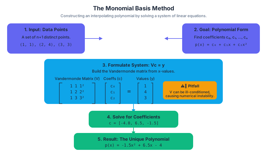
This system can be written in matrix form as Vc = y, where c is the vector of unknown coefficients, y is the vector of y_i values, and V is a special matrix known as the Vandermonde matrix.
\begin{pmatrix}
1 & x_0 & x_0^2 & \cdots & x_0^n \\
1 & x_1 & x_1^2 & \cdots & x_1^n \\
\vdots & \vdots & \vdots & \ddots & \vdots \\
1 & x_n & x_n^2 & \cdots & x_n^n
\end{pmatrix}
\begin{pmatrix}
c_0 \\
c_1 \\
\vdots \\
c_n
\end{pmatrix}
=
\begin{pmatrix}
y_0 \\
y_1 \\
\vdots \\
y_n
\end{pmatrix}
To find the coefficients, we simply need to solve this linear system for c.
Concrete Example
Let's find the quadratic polynomial that passes through the points (1, 1), (2, 4), and (3, 3). Here, n=2.
The Vandermonde system is:
V = [[1, 1, 1], [1, 2, 4], [1, 3, 9]]
y = [1, 4, 3]
The system of equations is:
c_0 + 1c_1 + 1c_2 = 1
c_0 + 2c_1 + 4c_2 = 4
c_0 + 3c_1 + 9c_2 = 3
Solving this system (e.g., using Gaussian elimination or a library function) yields c = [-4, 6.5, -1.5].
Thus, the interpolating polynomial is p(x) = -1.5x² + 6.5x - 4.
Implementation in Python
Solving a Vandermonde system is a standard task in numerical computing. Here is a Python implementation using NumPy.
import numpy as np

def monomial_interpolation_coeffs(x_points, y_points):
    """
    Computes the coefficients of the interpolating polynomial in the monomial basis.

    Args:
        x_points (np.ndarray): Array of x-coordinates of the data points.
        y_points (np.ndarray): Array of y-coordinates of the data points.

    Returns:
        np.ndarray: The coefficient vector [c_0, c_1, ..., c_n].
    """
    if len(x_points) != len(y_points):
        raise ValueError("x_points and y_points must have the same length.")

    n = len(x_points) - 1
    # np.vander creates the Vandermonde matrix with columns [x^n, x^(n-1), ..., 1]
    # We flip it to match our definition [1, x, ..., x^n]
    V = np.vander(x_points, increasing=True)

    # Solve the linear system Vc = y
    try:
        coeffs = np.linalg.solve(V, y_points)
        return coeffs
    except np.linalg.LinAlgError:
        raise RuntimeError("The Vandermonde matrix is singular. Check if x_points are distinct.")

# Example from the text
x_pts = np.array([1., 2., 3.])
y_pts = np.array([1., 4., 3.])

coeffs = monomial_interpolation_coeffs(x_pts, y_pts)
print(f"Coefficients (c0, c1, c2): {coeffs}") # Expected: [-4. ,  6.5, -1.5]

# To verify, let's evaluate the polynomial at x=2
p_at_2 = coeffs[0] + coeffs[1]*2 + coeffs[2]*2**2
print(f"p(2) = {p_at_2}") # Expected: 4.0
Common Pitfalls
The primary drawback of the monomial basis is numerical instability. For a high number of points, or for points clustered closely together, the Vandermonde matrix becomes ill-conditioned. An ill-conditioned matrix is one where small changes in the input y can lead to very large changes in the output solution c. This is because the columns of V, which are powers of x, become nearly linearly dependent for large n. The condition number of the matrix grows exponentially with n, making the solution highly sensitive to floating-point errors.
In practice, direct solution of the Vandermonde system is rarely used for n > 10.
The Lagrange Basis: An Elegant Theoretical Tool
The Lagrange basis offers a brilliantly clever way to construct the interpolating polynomial, completely bypassing the need to solve a linear system.
What It Is
The Lagrange basis consists of a set of n+1 polynomials, L_0(x), L_1(x), ..., L_n(x), each of degree n. These basis polynomials are defined with a special property related to the data points x_i.
Definition: Lagrange Basis Polynomials Each Lagrange basis polynomial
L_j(x)is defined as:L_j(x) = Π_{i=0, i≠j}^{n} (x - x_i) / (x_j - x_i)These polynomials have the "Kronecker delta" property:
L_j(x_k) = 1ifj=kand0ifj≠k.
How It Works
With this property, constructing the final interpolating polynomial p(x) becomes trivial. We form a linear combination of these basis polynomials, where the coefficients are simply the y_i values of our data points.
p(x) = Σ_{j=0}^{n} y_j * L_j(x)
Let's verify this works. If we evaluate p(x) at some x_k:
p(x_k) = Σ_{j=0}^{n} y_j * L_j(x_k)
Because L_j(x_k) is zero for all j≠k and one for j=k, all terms in the sum disappear except for one:
p(x_k) = y_k * L_k(x_k) = y_k * 1 = y_k
The polynomial passes through all points by construction.
Concrete Example
Using the same points (1, 1), (2, 4), (3, 3). Here x_0=1, x_1=2, x_2=3 and y_0=1, y_1=4, y_2=3.
- Construct
L_0(x):L_0(x) = ((x-x_1)(x-x_2)) / ((x_0-x_1)(x_0-x_2)) = ((x-2)(x-3)) / ((1-2)(1-3)) = (x²-5x+6)/2 - Construct
L_1(x):L_1(x) = ((x-x_0)(x-x_2)) / ((x_1-x_0)(x_1-x_2)) = ((x-1)(x-3)) / ((2-1)(2-3)) = (x²-4x+3)/(-1) - Construct
L_2(x):L_2(x) = ((x-x_0)(x-x_1)) / ((x_2-x_0)(x_2-x_1)) = ((x-1)(x-2)) / ((3-1)(3-2)) = (x²-3x+2)/2
The final polynomial is p(x) = y_0*L_0(x) + y_1*L_1(x) + y_2*L_2(x):
p(x) = 1 * (x²-5x+6)/2 + 4 * -(x²-4x+3) + 3 * (x²-3x+2)/2
Expanding and collecting terms gives p(x) = -1.5x² + 6.5x - 4, the same polynomial we found earlier.
Implementation in C
Here's a C function to evaluate a Lagrange polynomial at a specific point. This low-level implementation highlights the nested loop structure inherent in the formula.
#include <stdio.h>

// Evaluates the Lagrange interpolating polynomial at a single point 'x'.
double lagrange_evaluate(double x, const double* x_points, const double* y_points, int n) {
    double result = 0.0;

    // Outer loop for the sum: Σ y_j * L_j(x)
    for (int j = 0; j < n; ++j) {
        // Inner loop to compute L_j(x)
        double l_j = 1.0;
        for (int i = 0; i < n; ++i) {
            if (i != j) {
                l_j *= (x - x_points[i]) / (x_points[j] - x_points[i]);
            }
        }
        result += y_points[j] * l_j;
    }
    return result;
}

int main() {
    double x_pts[] = {1.0, 2.0, 3.0};
    double y_pts[] = {1.0, 4.0, 3.0};
    int n = sizeof(x_pts) / sizeof(x_pts[0]);

    // Evaluate at a few points to test
    printf("p(1.0) = %f\n", lagrange_evaluate(1.0, x_pts, y_pts, n)); // Expected: 1.0
    printf("p(2.0) = %f\n", lagrange_evaluate(2.0, x_pts, y_pts, n)); // Expected: 4.0
    printf("p(2.5) = %f\n", lagrange_evaluate(2.5, x_pts, y_pts, n)); // Expected: 4.375

    return 0;
}
Pitfalls and Variations
The main drawbacks of the Lagrange form are:
- Costly Evaluation: A naive evaluation, as shown in the C code, takes
O(n²)operations for each pointx. - Static Nature: If a new data point
(x_{n+1}, y_{n+1})is added, all Lagrange basis polynomials must be recomputed from scratch.
A significant improvement is the Barycentric Interpolation Formula, which is an algebraic rearrangement of the Lagrange form. It allows evaluation in O(n) time after an initial O(n²) pre-computation of weights. This makes it much more practical for repeated evaluations.
The Newton Basis: Efficient and Incremental
The Newton basis strikes a balance, offering both efficient evaluation and an elegant, incremental way to build the polynomial. It is often the most practical choice.
What It Is
The Newton form of the interpolating polynomial is:
p(x) = a_0 + a_1(x-x_0) + a_2(x-x_0)(x-x_1) + ... + a_n(x-x_0)...(x-x_{n-1})
The basis polynomials are π_j(x) = Π_{i=0}^{j-1} (x-x_i). The challenge is to find the coefficients a_0, a_1, ..., a_n.
How It Works: Divided Differences
The coefficients a_k are found using a recursive method called divided differences.
Definition: Divided Differences
- Zeroth divided difference:
f[x_i] = y_i - First divided difference:
f[x_i, x_{i+1}] = (f[x_{i+1}] - f[x_i]) / (x_{i+1} - x_i) - k-th divided difference:
f[x_i, ..., x_{i+k}] = (f[x_{i+1}, ..., x_{i+k}] - f[x_i, ..., x_{i+k-1}]) / (x_{i+k} - x_i)
The coefficients of the Newton polynomial are the top diagonal of the divided differences table:
a_k = f[x_0, x_1, ..., x_k]
This computation is typically organized in a triangular table.
Concrete Example
Let's use a new set of 4 points for clarity: (0, 1), (1, 4), (3, 40), (4, 85).
We build the divided differences table:
x_i |
f[x_i] (a₀) |
f[x_i, x_{i+1}] (a₁) |
f[x_i, ..., x_{i+2}] (a₂) |
f[x_i, ..., x_{i+3}] (a₃) |
|---|---|---|---|---|
| 0 | 1 | |||
(4-1)/(1-0) = 3 |
||||
| 1 | 4 | (18-3)/(3-0) = 5 |
||
(40-4)/(3-1) = 18 |
(7-5)/(4-0) = 0.5 |
|||
| 3 | 40 | (45-18)/(4-1) = 9 |
||
(85-40)/(4-3) = 45 |
||||
| 4 | 85 |
The coefficients are the top entries: a_0=1, a_1=3, a_2=5, a_3=0.5.
The polynomial is:
p(x) = 1 + 3(x-0) + 5(x-0)(x-1) + 0.5(x-0)(x-1)(x-3)
Algorithm and Library Usage
The process of computing the divided differences is algorithmic.
function DividedDifferences(x_points, y_points):
    n = length(x_points)
    // Initialize a table (e.g., a 2D array)
    table = new array of size n x n

    // The first column is just the y-values
    for i from 0 to n-1:
        table[i][0] = y_points[i]

    // Compute the rest of the table
    for j from 1 to n-1: // Column index
        for i from 0 to n-1-j: // Row index
            numerator = table[i+1][j-1] - table[i][j-1]
            denominator = x_points[i+j] - x_points[i]
            table[i][j] = numerator / denominator

    // The coefficients are the first row of the table
    return table[0]
In practice, high-quality numerical libraries provide robust implementations. SciPy's BarycentricInterpolator uses a related form and can be updated efficiently.
import numpy as np
from scipy.interpolate import BarycentricInterpolator
import matplotlib.pyplot as plt

# Data points
xi = np.array([0., 1., 3., 4.])
yi = np.array([1., 4., 40., 85.])

# Create the interpolator object
poly = BarycentricInterpolator(xi, yi)

# Let's add a new point to demonstrate the incremental nature
# This is a key advantage of Newton-like forms
new_x, new_y = 2.0, 15.0
poly.add_xi(np.array([new_x]), np.array([new_y]))

# Generate points for plotting a smooth curve
x_dense = np.linspace(-0.5, 4.5, 400)
y_dense = poly(x_dense)

# Plot the results
plt.style.use('seaborn-v0_8-whitegrid')
plt.figure(figsize=(10, 6))
plt.plot(x_dense, y_dense, label='Newton Interpolating Polynomial (with added point)')
plt.plot(xi, yi, 'ro', label='Original Points')
plt.plot(new_x, new_y, 'go', markersize=10, label='Added Point (2, 15)')
plt.title('Newton Interpolation with Incremental Update')
plt.xlabel('x')
plt.ylabel('y')
plt.legend()
plt.show()
Efficient Polynomial Evaluation: Horner's Method
Regardless of how we find the coefficients c_i for the monomial form p(x) = c_0 + c_1x + ... + c_nx^n, evaluating it efficiently is critical. A naive evaluation requires O(n²) multiplications (computing x^k for each term). Horner's Method is an elegant algorithm that reduces this to O(n).
How It Works
Horner's method works by refactoring the polynomial into a nested form. For a degree 4 polynomial:
p(x) = c_0 + c_1x + c_2x² + c_3x³ + c_4x⁴
p(x) = c_0 + x(c_1 + x(c_2 + x(c_3 + x(c_4))))
This nested structure can be evaluated from the inside out with a simple loop, requiring only n multiplications and n additions.
Implementation in JavaScript
This algorithm is simple and efficient, making it suitable for implementation in any language. Here's a JavaScript example.
/**
 * Evaluates a polynomial in monomial form using Horner's method.
 * @param {number[]} coeffs - Array of coefficients [c0, c1, ..., cn].
 * @param {number} x - The point at which to evaluate the polynomial.
 * @returns {number} The value of the polynomial at x.
 */
function horner(coeffs, x) {
    // Start with the highest-degree coefficient
    let result = coeffs[coeffs.length - 1];

    // Iterate backwards from the second to last coefficient
    for (let i = coeffs.length - 2; i >= 0; i--) {
        result = result * x + coeffs[i];
    }

    return result;
}

// Example: p(x) = -1.5x² + 6.5x - 4  (coeffs are [-4, 6.5, -1.5])
const myCoeffs = [-4, 6.5, -1.5];
console.log(`p(1) = ${horner(myCoeffs, 1)}`); // Expected: 1
console.log(`p(2) = ${horner(myCoeffs, 2)}`); // Expected: 4
console.log(`p(3) = ${horner(myCoeffs, 3)}`); // Expected: 3
The Problem with High-Degree Polynomials: Runge's Phenomenon
A common misconception is that using more data points (and thus a higher-degree polynomial) will always lead to a better approximation of the underlying function. This is dangerously false. High-degree polynomial interpolants can exhibit wild oscillations, especially near the ends of the interpolation interval.
This behavior is known as Runge's phenomenon, famously demonstrated with the function f(x) = 1 / (1 + 25x²). When interpolating this function on the interval [-1, 1] with equally spaced points, the error between the true function and the interpolating polynomial p_n(x) grows dramatically as n increases.
The error of polynomial interpolation is given by:
f(x) - p_n(x) = (f^(n+1)(ξ) / (n+1)!) * Π_{i=0}^{n} (x - x_i)
where ξ is some point in the interval.
Two factors contribute to Runge's phenomenon:
- The derivatives of Runge's function grow very rapidly.
- The product term
Π(x - x_i)becomes very large near the endpoints for equally spaced points.
Solution: Chebyshev Points
The magnitude of the error can be controlled by changing the locations of the x_i points. The optimal choice to minimize the maximum error are the Chebyshev points, which are clustered more densely near the ends of the interval.
They are defined on [-1, 1] as:
x_i = cos( (2i+1)π / (2n+2) ) for i = 0, ..., n.
Using Chebyshev points instead of equispaced points dramatically mitigates Runge's phenomenon and guarantees convergence for a wide class of functions.
Piecewise Interpolation: The Practical Solution
Instead of using a single, high-degree polynomial to fit all data points, a more robust and widely used approach is piecewise interpolation. The idea is to divide the interval into smaller subintervals and fit a separate, low-degree polynomial on each piece. The collection of these polynomials is called a spline.
How It Works
- Piecewise Linear Interpolation: Simply connect consecutive data points with straight lines. The resulting function is continuous (
C⁰) but has sharp corners (its derivative is not continuous). - Piecewise Cubic Splines: The most common choice. We fit a cubic polynomial between each pair of points
(x_i, y_i)and(x_{i+1}, y_{i+1}). To ensure smoothness, we add constraints that the first and second derivatives must match at the "knots" (the data points). This results in a function that is twice continuously differentiable (C²), making it visually smooth and well-behaved.
Why It Matters
Splines avoid Runge's phenomenon entirely because they only ever use low-degree polynomials. They are stable, efficient to compute, and provide excellent approximations for most real-world data. They are the workhorse of interpolation in computer graphics, data visualization, and scientific computing.
| Method Comparison | Construction Cost | Evaluation Cost | Stability | Key Feature |
|---|---|---|---|---|
| Monomial Basis | O(n³) |
O(n) |
Poor | Simple representation, but ill-conditioned. |
| Lagrange Basis | O(n²) |
O(n²) |
Fair | Trivial coefficients, theoretically elegant. |
| Newton Basis | O(n²) |
O(n) |
Good | Incremental updates, numerically stable. |
| Cubic Splines | O(n) |
O(log n) |
Excellent | Avoids oscillations, provides C² smoothness. |
Source Materials
Study CS323: Numerical Analysis and Computing on Lykke
This course page is free to open: signed out, you can read its first two sections, and signing in, on any plan, opens the rest. The free Lykke Chrome extension syncs your own Canvas courses, so ChatGPT, Claude and Muse can answer from your classes and deadlines. It only reads Canvas.
Add the free extensionSign in to open every sectionAll sections of CS323: Numerical Analysis and Computing · Browse more course pages